Essence of A/B testing - notes

Objective

I like to share the core concepts which repeats itself in different flavors of hypothesis testing focussing on classic frequentists approach of A/B or split testing.

Non-objective

I will be alluding to Bayesian inference and techniques for hypothesis testing but not go deep in this post. In the future post, I may write about topics related to Bayesian inference related topics. This post is a way to share my notes and it won’t cover pitfalls of frequentists approach of A/B testing.

Confidence interval, central limit theorem, z-dist, z-values

The following concepts of z-distribution, confidence interval, central limit theorem plays an important role in frequentist approach of A/B testing.

Z-distribution

Z-distribution: The Standard Normal Distribution

The z-distribution, also called the standard normal distribution, is a specific type of normal distribution with two key characteristics:

Mean (μ) of 0 Standard deviation (σ) of 1

Confidence interval

Let’s say you flipped the coin 20 times (your sample) and got 12 heads (sample mean). You want to estimate the likelihood of the actual population mean (fairness of the coin) falling within a certain range.

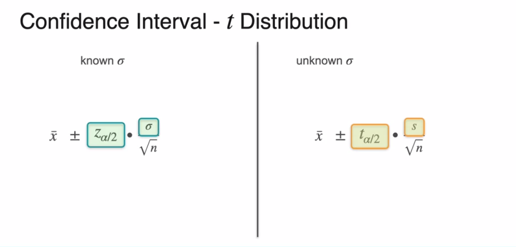
This is where confidence intervals come in. They use the z-distribution or t-distribution(comes later in post) to provide a range of values where the population mean is likely to reside, based on your sample data. Here’s the formula:

Sample mean ± (z-score * standard error) (using z-distribution)

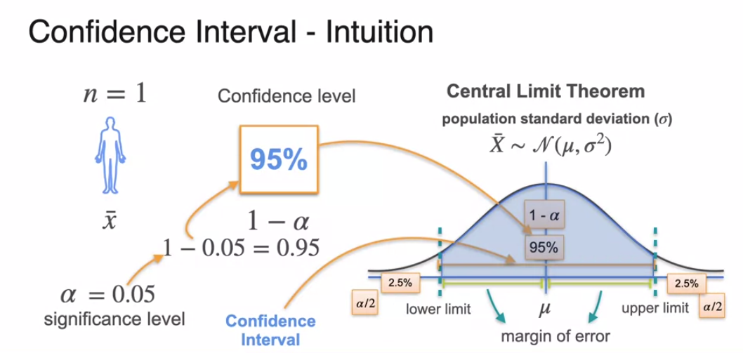
The z-score depends on your chosen confidence level (e.g., 95% confidence means a 2.5% chance the true mean falls outside the interval). The standard error is the estimated standard deviation of the sampling distribution, calculated using the sample standard deviation and sample size.

pb-basics

Central limit theorem

Confidence intervals rely on information from a sample to make inferences about an entire population. However, the challenge is that most real-world populations don’t necessarily follow a normal distribution (like the familiar bell curve). Central limit theorem comes to the rescue! It tells us that under certain conditions, the distribution of averages (means) from random samples, regardless of the original population’s shape, will tend towards a normal distribution as the sample size increases.

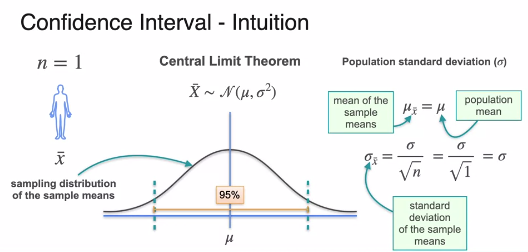
From the central limit theorem, you know that if you were to take multiple samples of this size and create a sampling distribution for the sample means for a sample of size 1. The sampling distribution of the sample means makes a gaussian with a center at mu and a standard deviation of sigma.
The concept of the confidence interval is heavily tied to the fact that we’re taking multiple samples off a certain size to get a sampling distribution of sample means, where with large samples, the sampling distribution tends towards a Gaussian of the form x bar. If we were to standardize the distribution, we’d let Mu = 0 and Sigma be 1.
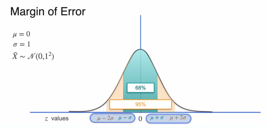
Recall that when a normal distribution is standardized, then 68% of the population falls one standard deviation away from the mean, whereas 95% falls two standard deviations away from the mean. These values over here are called the z values.

Margin of error:

pb-basics

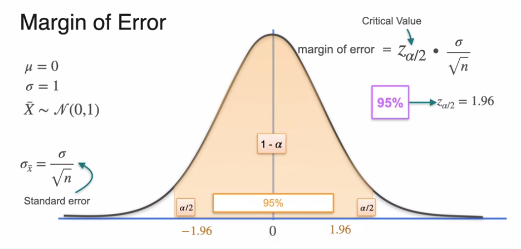
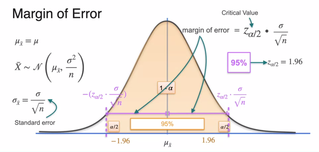
Notice that the lower and upper limits are just some standard deviation value away from the true mean. But these standard deviation intervals defined by the confidence level we choose, essentially is something we call the margin of error. And by adding the margin of errors to any sample mean from the sample distributions, we get the confidence interval.
Now, multiplying the standard error with the critical value, you get the margin of error as you’re essentially scaling the distribution with a standard deviation while using the critical values to capture the upper and lower limits where 95% of the distribution will lie. The center of this distribution is the population mean for the sampling distributions. You then have these margins that indicate an interval where 95% of the time the interval captures the population mean.

Unknown standard deviation

| What if the population standard deviation is unknown?

Student t-distribution

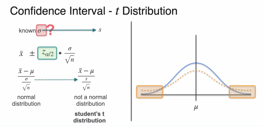
Using the normal distribution as a reference. The Student t-distribution looks like this. It’s very similar to a normal distribution, but it has much fatter tails, meaning that more of the points can be found on these sides compared to the normal distribution. If you were to sample a point out of the Student t-distribution is more likely to be far from the center than if you pick it from the normal distribution.
There can be several t-distributions defined by something we call the degree of freedom. The degree of freedom of a t-distribution is given by the number of samples that we used minus 1.
Degree of freedom varies for two sample t-test which you will see later in the post.
The degree of freedom defines how high and tight the t-distribution is.
The larger the number of degrees of freedom, the closer and closer you get to a normal distribution. This makes sense because the more samples you use, the bigger n is, the closer and closer that your sample standard deviation s is to the population standard deviation Sigma. If you know Sigma, you use a normal distribution. The closer you get to Sigma, the closer you get to using a normal distribution.

pb-basics

In the context of hypothesis testing

stats

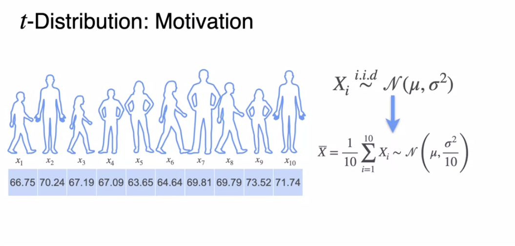
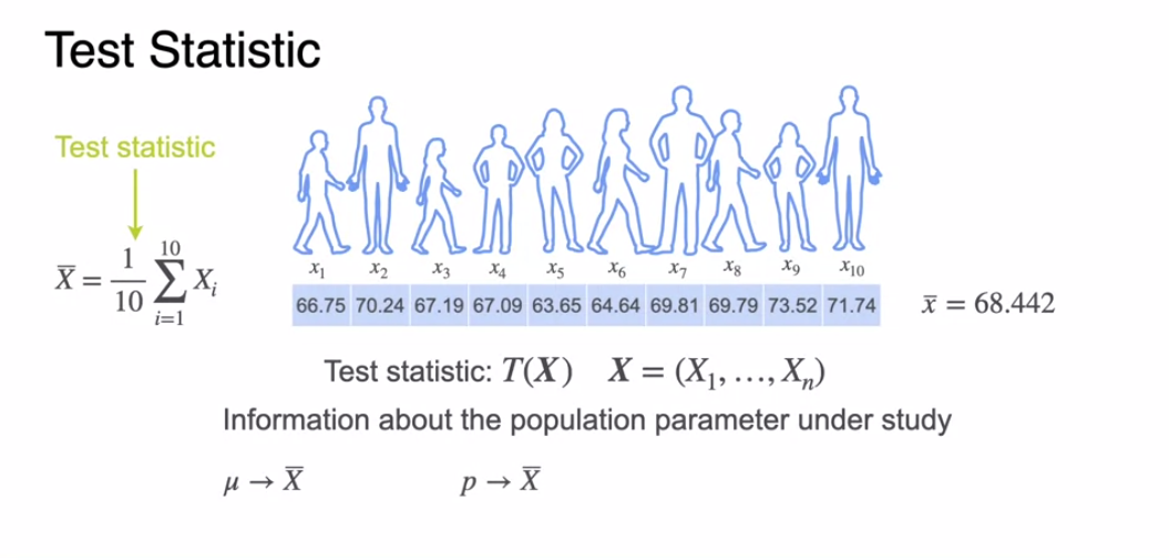
Consider the example of sampling the height of 10 18-year-olds. Recall, people’s heights can be modeled as a Gaussian distribution with parameters Mu and Sigma. As a consequence, the sample mean will follow a Gaussian distribution of the same mean, but a smaller standard deviation, because now we have 10 samples.

stats

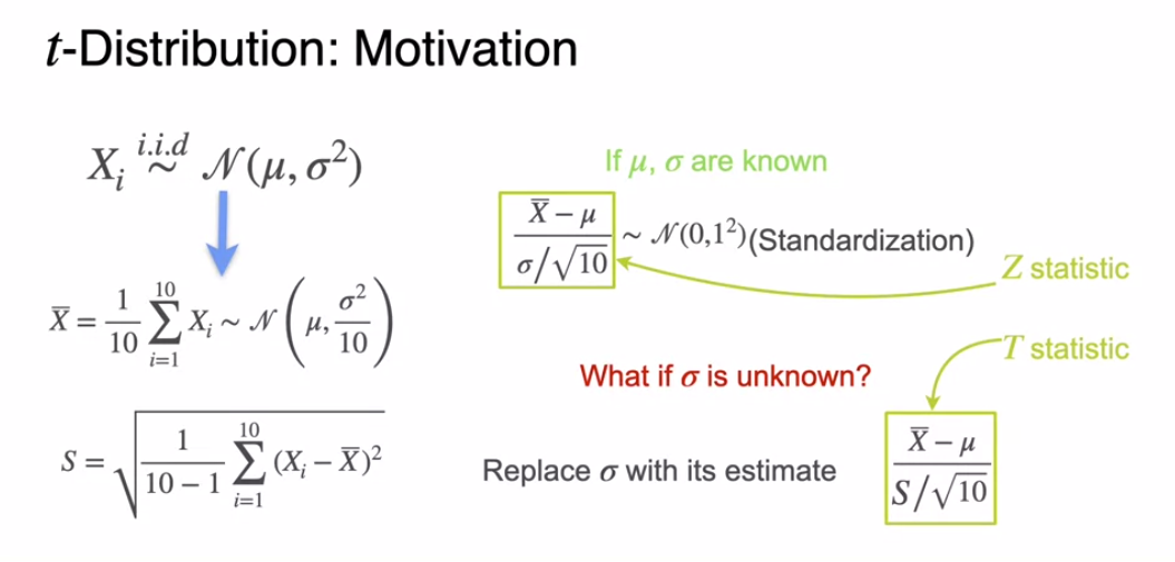
Well, if Mu and Sigma are known, then you already learned that the sample mean minus Mu divided by the sample standard deviation follows a standard normal distribution. This is simple standardization. This statistic is called the Z statistic. But what if Sigma is unknown, which is the more common case? Then knowing that the sample mean is a Gaussian with standard deviation Sigma over square root of 10 is not very useful because you don’t know what the value of Sigma is. What you do you do in this case is to replace the value Sigma in the standardization formula by its estimate .
S can defined as almost the variance of the sample, except you divide it by n-1 instead of n. It is the square root of the sum of squared difference between the sample and the sample mean divided by n-1. The resulting statistic is called the t statistic.
Recall, t statstics doesn’t follow standard normal distribution but student t-distribution or t-distribution.
The degree of freedom is independent of the population mean and variance and only depends upon the number of samples you collected.

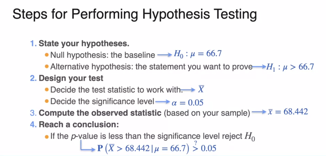
Hypothesis

| Null-hypothesis H-0 - base assumption

| Alternative-hypothesis H-1 - represents the competing statement. And given the asymmetry and the conclusions, this is usually the one you’re interested in proving. And the goal of hypothesis testing is deciding between two hypotheses based on data and evidence.

Type-1 and type-2 errors

stats

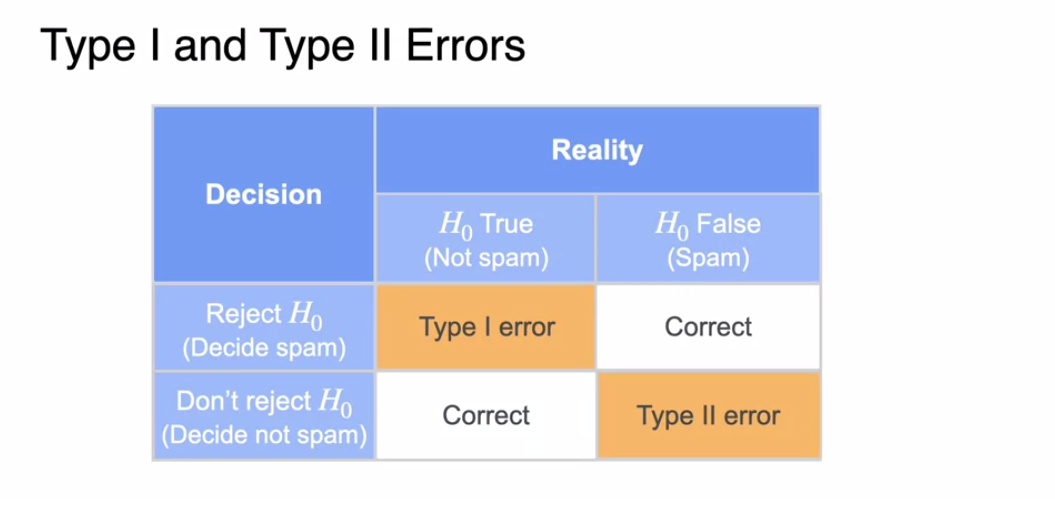
It is important to remember the following defenitions of false positive and false negative which is related to upcoming p-value and beta sections.

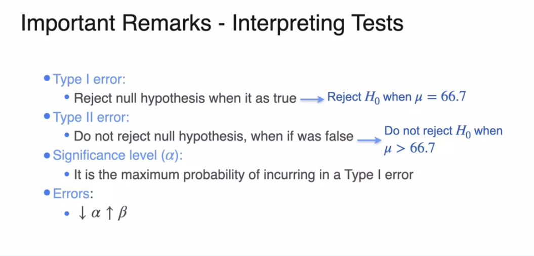
| Type-1 error - Rejecting null hypothesis which is actually true

| Type-2 error - Failing to reject null hypothesis which is actually false

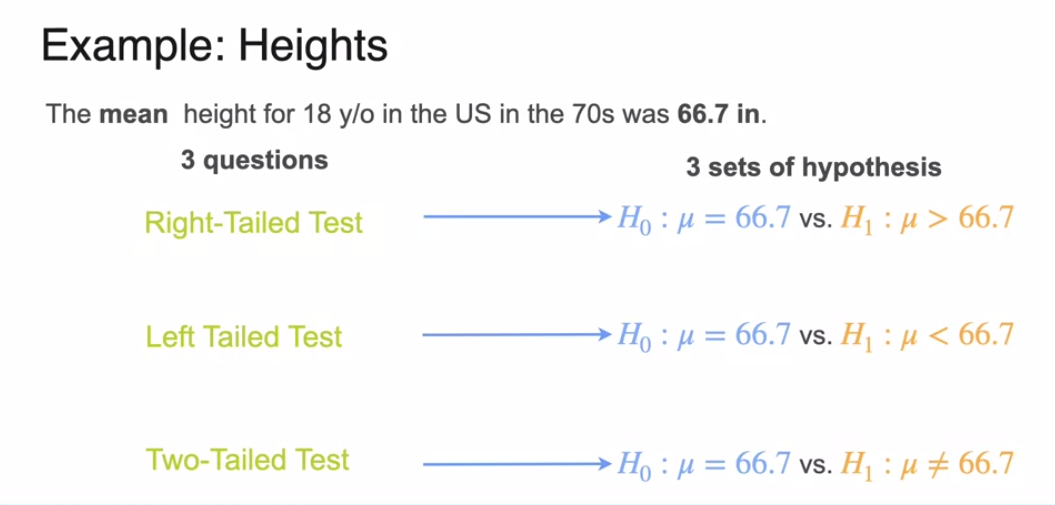
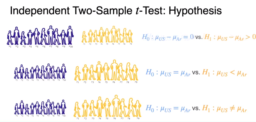
Left tailed, right tailed and 2-tailed tests

stats stats stats stats

p-value (statistical significance)

stats stats stats

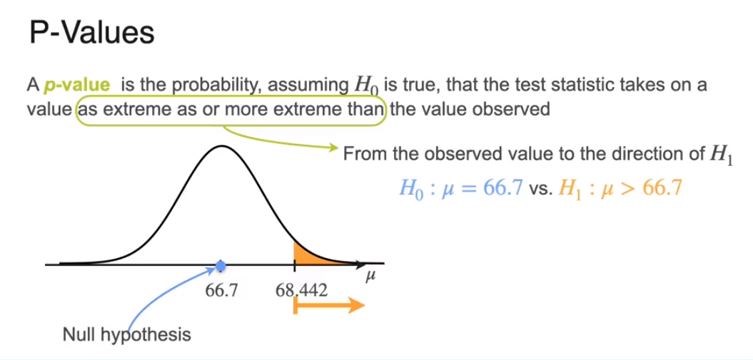
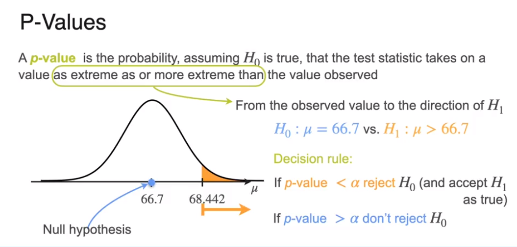
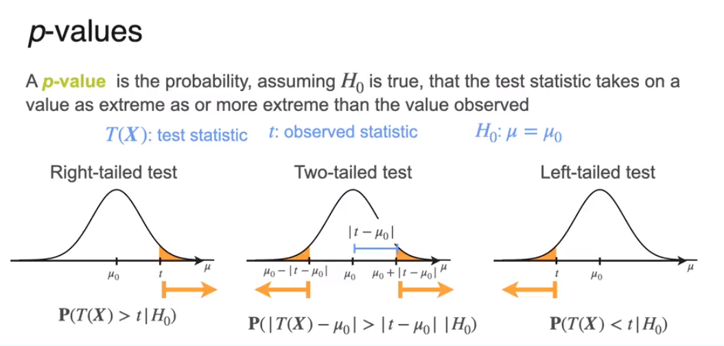
Once the test statistic is calculated, p-value can be calculated programatically using libraries like Scipy, Statsmodel.

Power of test and Beta

stats stats

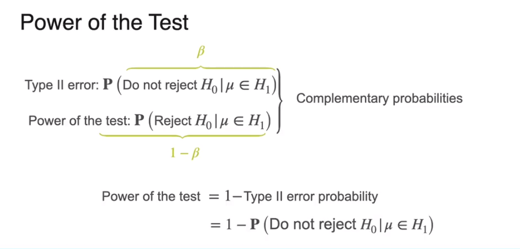
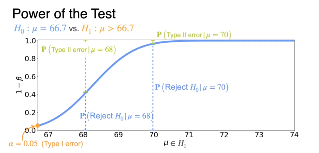
Recall

stats stats stats

Two sample t-test

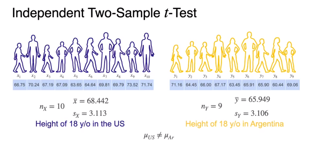
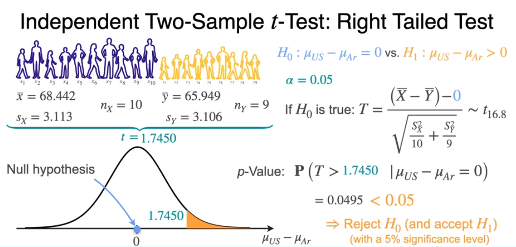
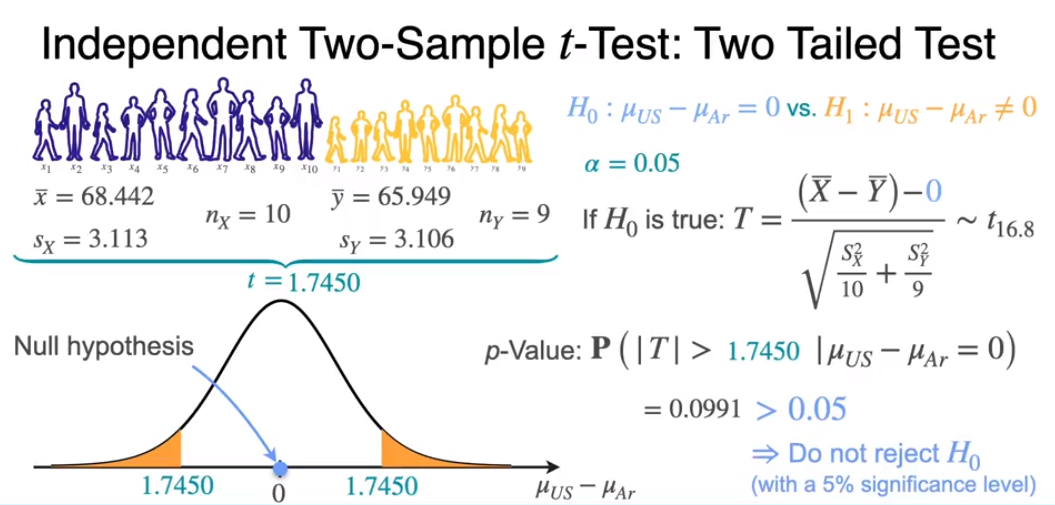
Consider for this example that you’re interested in comparing the heights of 18 year olds in the US with the heights of 18 year olds in Argentina. The first group, you have 10 samples x1 upto x_10, which with the values shown above, have an observed sample mean of 68.442 inches and a sample standard deviation of 3.113. For the Argentinian group, you have only nine samples, y 1 upto y_9 with an observed mean of 65.949 inches and a sample standard deviation of 3.106 inches. Your goal is to determine if the population mean from the US is different than the population mean from Argentina.

stats stats stats

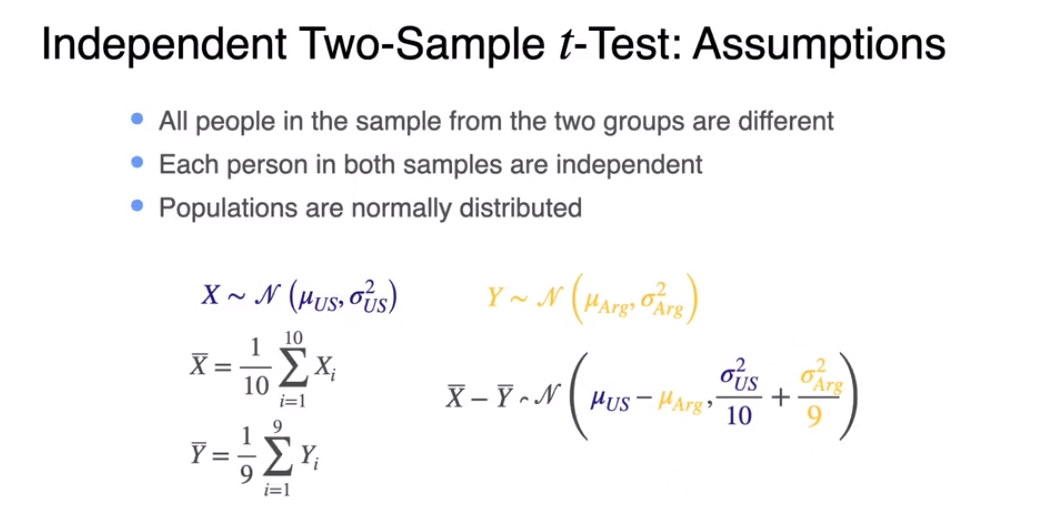
How does the difference between both sample means distribute? Since it’s a linear combination of Gaussian variables, then it will also be a Gaussian, but with which parameters? The mean will be the difference of the population means and the standard deviation will be the square root of the variances of each sample mean.

stats stats

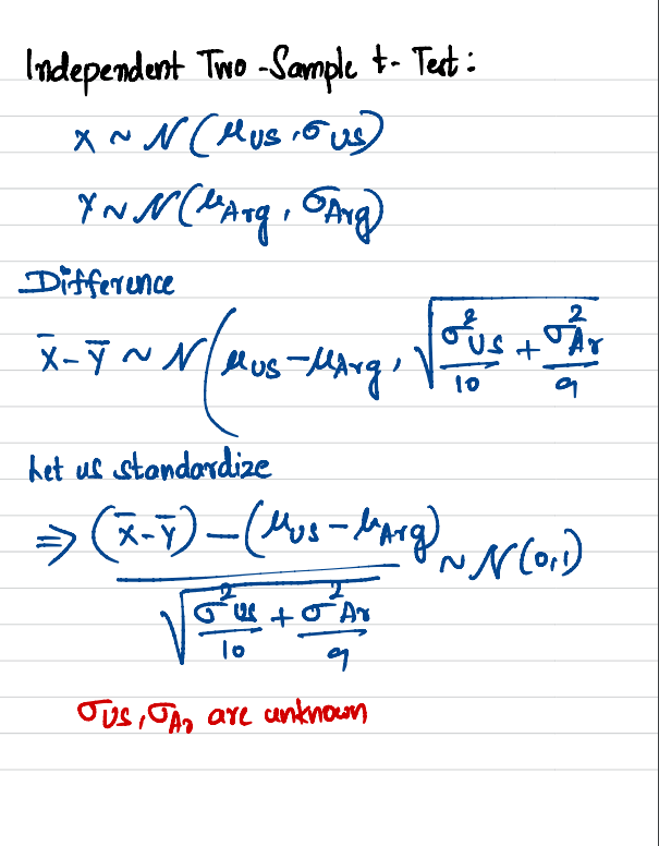
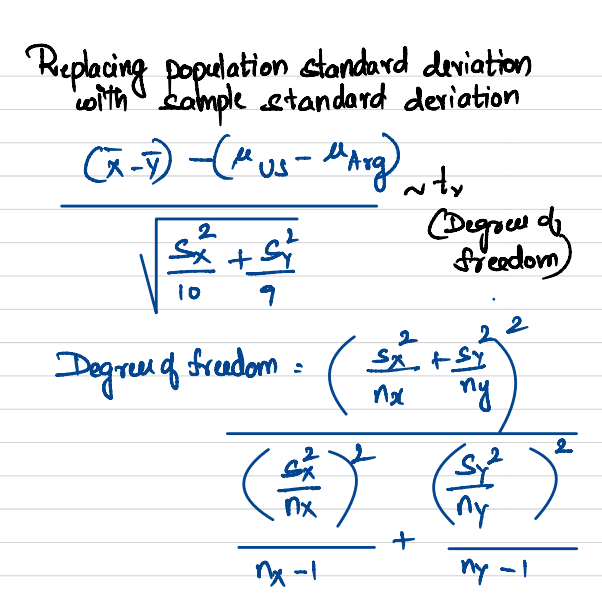
Once test statistic is derived and observed statistic can be calculated with the observation, we can calculate the p-value.
p-value can be compared with significance level to make decision on whether to reject null hypothesis or not. The following are based on right tailed test and two tailed test.

stats stats

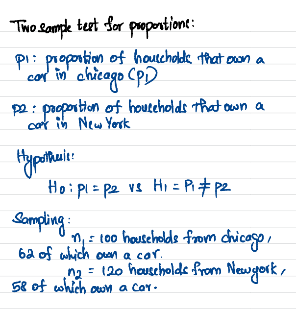
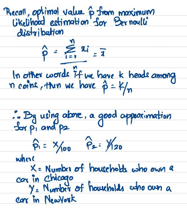
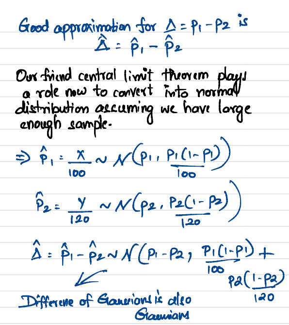
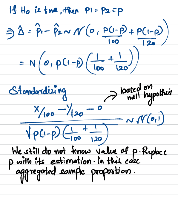
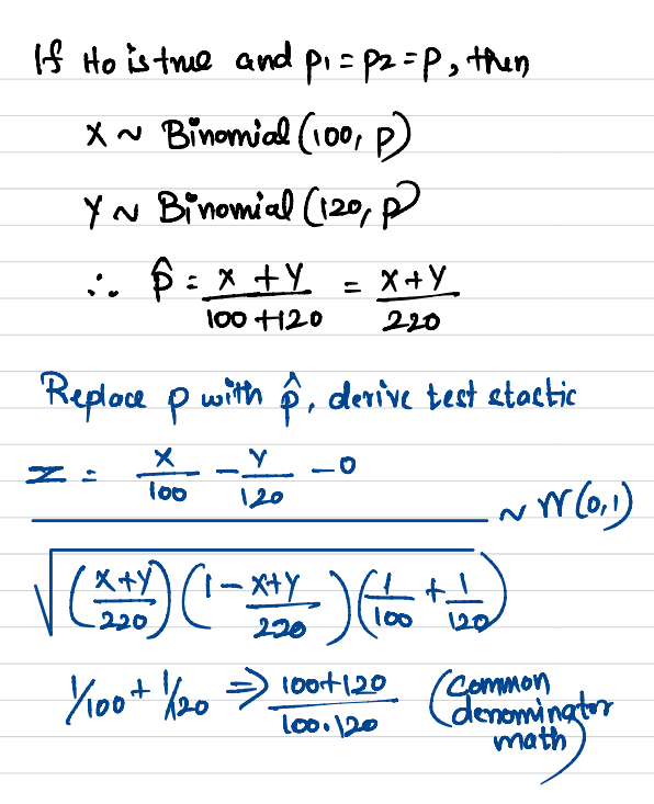
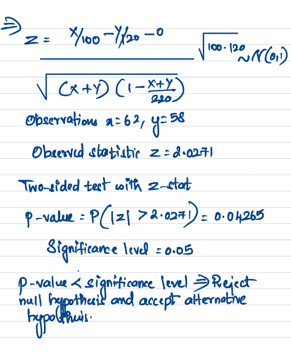
Two sample t-test for proportion from two different population.

Its an important section as well before we look full fledged application of hypothesis testing (testing statistical significance) of both continous metric and discrete metric.

stats stats stats stats stats stats

A/B Testing/Culture of experimentation

| Refer to my completed notebook (link below) checked in to Gitlab for code samples on A/B testing for both continous metric and proportion metric.

Following are my favorite highlights from my favorite company Netflix. Please check for references below.

Running A/B tests, wherever possible, allows us to substantiate causality and confidently make changes to the product knowing that our members have voted for them with their actions.
The goal here is to articulate the causal chain, from how user behavior will change in response to the new product experience to the change in our primary decision metric.
Articulating the causal chain between the product change and changes in the primary decision metric, and monitoring secondary metrics along this chain, helps us build confidence that any movement in our primary metric is the result of the causal chain we are hypothesizing, and not the result of some unintended consequence of the new feature
how we turn an idea into a testable hypothesis
It’s important to acknowledge that no approach to decision making can entirely eliminate uncertainty and the possibility of making mistakes. Using a framework based on hypothesis generation, A/B testing, and statistical analysis allows us to carefully quantify uncertainties, and understand the probabilities of making different types of mistakes.
There are two types of mistakes we can make in acting on test results. A false positive (also called a Type I error) occurs when the data from the test indicates a meaningful difference between the control and treatment experiences, but in truth there is no difference. This scenario is like having a medical test come back as positive for a disease when you are healthy. The other error we can make in deciding on a test is a false negative (also called a Type II error), which occurs when the data do not indicate a meaningful difference between treatment and control, but in truth there is a difference. This scenario is like having a medical test come back negative — when you do indeed have the disease you are being tested for.
The uncomfortable truth about false positives and false negatives is that we can’t make them both go away. In fact, they trade off with one another. Designing experiments so that the rate of false positives is minuscule necessarily increases the false negative rate, and vice versa. In practice, we aim to quantify, understand, and control these two sources of error.
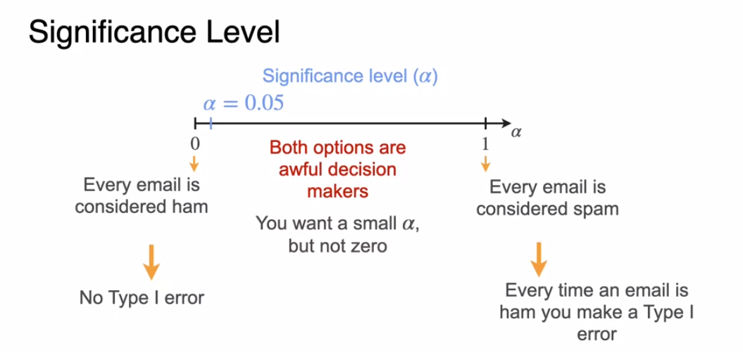
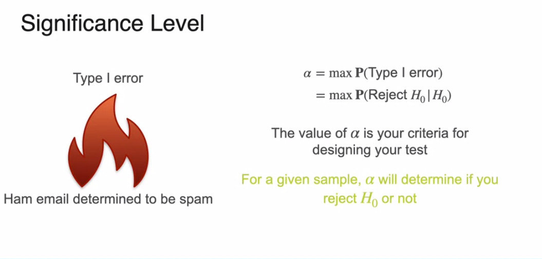
With a great hypothesis and a clear understanding of the primary decision metric, it’s time to turn to the statistical aspects of designing an A/B test. This process generally starts by fixing the acceptable false positive rate. By convention, this false positive rate is usually set to 5%: for tests where there is not a meaningful difference between treatment and control, we’ll falsely conclude that there is a “statistically significant” difference 5% of the time. Tests that are conducted with this 5% false positive rate are said to be run at the 5% significance level.
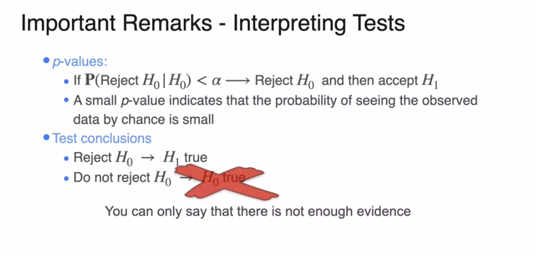
The p-value is the probability of seeing an outcome at least as extreme as our A/B test result, had there truly been no difference between the treatment and control experiences.
It’s a lot like a jury trial, where the two possible outcomes are “guilty” or “not guilty” — and “not guilty” is very different from “innocent.” Likewise, this (frequentist) approach to A/B testing does not allow us to make the conclusion that there is no effect — we never conclude the coin is fair, or that the new product feature has no impact on our members. We just conclude we’ve not collected enough evidence to reject the null assumption that there is no difference.