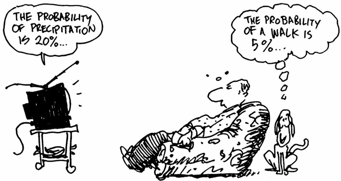
#My favorite topics and notes on probability (in context of machine and deep learning)

This post is part of yet another series. My goal is to share some of topics which caught my attention immediately when I was going through some of the common materials.

#Key objectives

• We know fitting line to data and finding the best line by optimizing the squared error loss function to find the optimal parameters for the best line which fits the data perfectly. In this post, we can see a different probability perspective to find the highest probability that a particular model among other models produced the datasets.
• As we saw in calculus post, about optimizing loss functions by taking partial derivatives and finding the best parameter by solving partial derivatives based on parameters equated to zero. In this post, I like to highlight an approach of viewing the probability distribution function as function of respective parameters and solving them in similar fashion to above said point to find the maximum likelihood.
• Bayesics - This post is yet another post. However, I reiterate in my own words about importance and beauty of conditional probability, Bayesians view of probability and how prior probabilities plays an important role. Last but not least, I will share few highlights on my favorite topic relating maximum likelihood estimation, regularization, generalized version of maximum likelihood estimation using Bayes rule called as maximum a posterior estimation (MAP).

#Machine Learning + Probability

• I am specializing in Natural language processing and understanding, also Generative Adversial Networks. In future posts, I will highlight specifically. In this post, I like to talk about importance of conditional probability and maximing pure probabilities in machine, deep learning topics.

• Sentiment Analysis - P ( Positive or Negative or Neutral | words in the sentence) => Conditional probability of sentiment given set of words in the sentence.

• Image Analysis - P ( Cat | pixel 1…n) => Conditional probability that image is a cat conditioned on given input pixels.

• Health care - P (Healthy or Unhealthy | symptoms and history) => Is the patient healthy or unhealthy conditioned on symptoms and history. Yet another conditional probability.

• My favorite StyleGAN (Face Generation) => as an example of maximizing pure probability. Generate group of pixels, such the resulting image looks like human face. Goal is to maximize the probability P (face | pixels) and generate images with highest probability.

#Basics Revisited

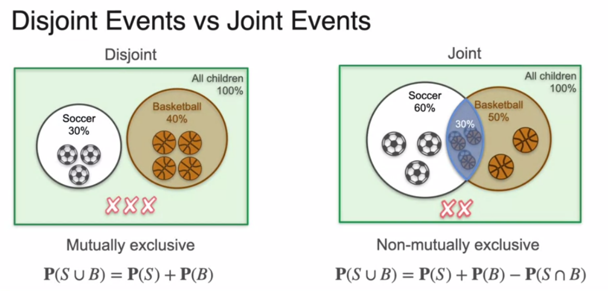
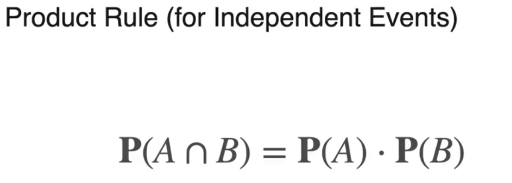
In my calculus post or any calculus posts will talk about basic rules like sum, product rule, chain rule which becomes part of daily life of calculus practitioners. In a similar way, in probability, we have certain every day rules like sum of probabilities (disjoint events, joint events), product rule (independent events) and conditional probability - where sequential events depend on each other, espcially second event depeneding on prior event, we have product of events.

| In this post, you will see me over communicating or insisting on conditional probability heavily

#Independent Events - In machine learning, if events are independent to each other or if we can assume they are independent; it makes certain topics easy as calculation of probability of independent events becomes easy by product rule.

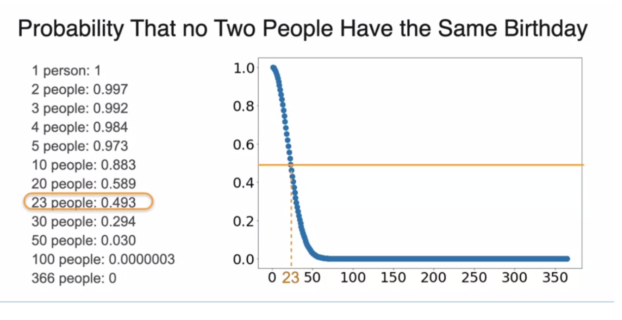
• Best example of independent events and easeness to calculate probability when they are independent is birthday problem. The problem is, we have group of friends in the party. What is more likely? 1) There exists two people with same birthday 2) No two of them have same birthday.

In the following, the first person has chance of 365/365 (365 days in a year) as birthday. The second person has 364 days / 365 days, remaining 364 days/365 as probability and it follows for the rest of the people in group. As they are independent events, the total probability is just a product of events.

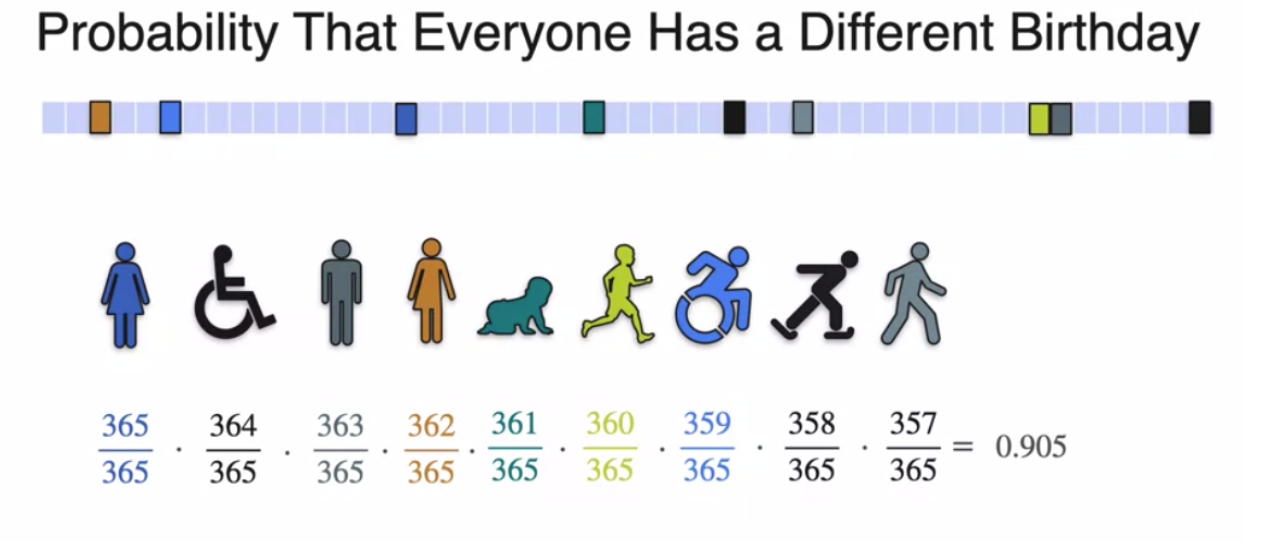
When we plot the probability calculated for a different number of people in the group all the way from group of one, we get the following which helps us to bet. For example, in a group of 23 people, we can win more than half of times guessing that two people in the group have same birthday in a year.

#Conditional Probability

• Conditional probability is all about calculating the probability of an event happening given that another event has already happened.

• In this post, I like to highlight two important facts about conditional probability.

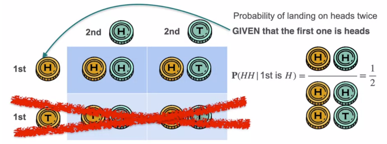
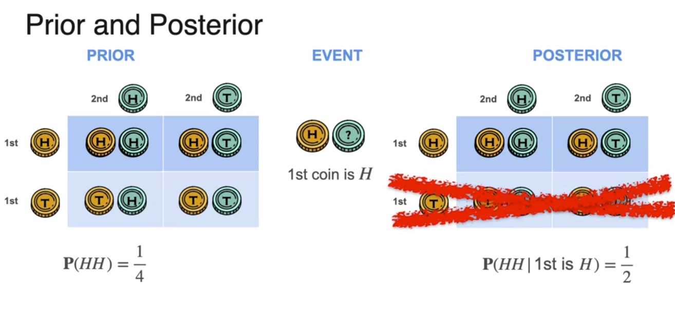
  • Without talking early about jargons like prior, posterior or event, let me share the fact that conditional probability helps to reduce the sample space. I have included classic example with coin toss. Sample space reduces when we are aware of an event which can impact the next event for which we are interested to calculate the probability. In the following example of classic coin toss, since there is a condition first coin toss results in heads, we can see that sample space has reduced.

  

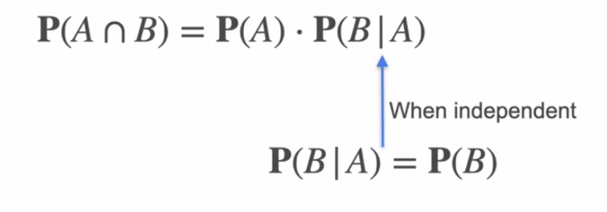
  • The second fact which I like to highlights is about general product rule which applies to independent events changes slightly for conditional probability when sequential events depend on each other.

  

  #Monty Hall problem

  Image Credit - Wikipedia

  Why am I talking about movie 21? Have you watched it? The first challenge professor (actor) gives in his MIT class is Monty Hall problem. One of my favorite movies. Again, conditional probablity shines and informs us that condition or extra information always gives us better probability. To be precise, posterior probability is better than prior because of the extra information. In the above movie scene or Monty Hall problem, we can the effect of using extra information. Lets see the analytical version below.

#Problem

Suppose you are in a TV show where you may win a car by playing a game. The game is very simple: you have to choose among three closed doors. One door has the car and the other two have goats.

The game is played in two steps:

1) The host lets you choose one among the three doors, but you do not open it yet. 2) Then, the host (who knows where the car is) choose one among the two remaining doors and open it, revealing a goat.

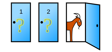
Monty Hall Problem - from Wikipedia

The time to choose has come and let’s suppose you have chosen door number 1. Then, just before they open the door number 1, the Host - who already knows in which door the car is behind - opens door number 3, revealing a goat and leaving doors number 1 and 2 closed. The Host then asks you:

“Would you like to switch your choice to door number 2?”

Define the events:

𝐸1 = the car is behind door 1
𝐸2 = the car is behind door 2
𝐸3 = the car is behind door 3

Or, in a more concise way:
𝐸𝑖 = the car is behind door 𝑖, for 𝑖=1,2,3 . Note that these events are mutually exclusive, in other words, you cannot have a car simuntaneously in two doors, because of the rules of the game. This means that,

𝑃(𝐸1∩𝐸2)=0, 𝑃(𝐸1∩𝐸3)=0 and 𝑃(𝐸2∩𝐸3)=0 𝑃(𝐸𝑖∩𝐸𝑗)=0 for 𝑖≠𝑗.

Another fact, due to the rules of the game, is that the car is behind one of the three doors, so

𝑃(𝐸1 ∪ 𝐸2 ∪ 𝐸3)=1.

This is, in fact, the sample space, or universe, Ω, because it is the set of all possible outcomes.

Let’s suppose you’ve chosen door number 1. Since there is an equal chance of the car being behind one of the three doors, we know that 𝑃(𝐸1) = 1 / 3.

By the complement rule, we know that 𝑃(𝐸𝑐1) = 1−𝑃(𝐸1) = 1−(1/3) = 2/3

Since the universe is given by 𝐸1 ∪ 𝐸2∪ 𝐸3 (the car is behind door 1 OR door 2 OR door 3), then 𝐸𝑐1 = 𝐸2 ∪ 𝐸3, therefore 𝑃(𝐸2∪𝐸3)=2/3. You can have a visual idea in the image below.

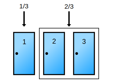
Monty Hall Closed Doors - from Wikipedia

Now that you chose door 1, the Host then opens door 3, revealing a goat and asks you if you want to switch doors. If you don’t switch, the probability of winning remains 1/3 because this is your initial choice. If you do switch, then, you can notice that the Host gave you an additional information. They showed to you that door 3 does not have a car, which means that

𝑃(𝐸3)=0.

Now you are mostly done, because as you know, 2 / 3 = 𝑃(𝐸2∪𝐸3) = 𝑃(𝐸2)+𝑃(𝐸3)−𝑃(𝐸2∩𝐸3). You already know that 𝑃(𝐸2∩𝐸3)=0 because they are mutually exclusive events (the car is behind in only one of the three doors), and the Host gave you a very importante piece of additional information: 𝑃(𝐸3)=0. With this, you can easily conclude that:

𝑃(𝑤𝑖𝑛|𝑠𝑤𝑖𝑡𝑐ℎ) = 𝑃(𝐸2) = 2/3.

In other words, the probability that the car is behind door 2, given that it is not behind door 3 is 2/3 ≈ 0.67

#Bayes

One of my favorite topics in Probability is classic Bayes Theorem since it depends on my favorite conditional probability. Our life itself is conditioned on something most of the time.

I like to share my notes of following related to Bayes

• #Setting foundation to derive Bayes formula

• #Bayes formula - highlights

• #Naive Bayes model

TO-DO - Checking the notebook to Gitlab (on Bayes)

#Setting foundation to derive Bayes formula (again conditional probability facts above plays major role)

Image credit: uchicagomedicine

Before I share facts about Bayes formula, lets set foundation. We have been through Covid-19 pandemic which affected the world population. We either feel sick and wanted to get tested. Again conditional probability of testing positive when you know you are sick and show symptoms. In other way, lets assume there is a test with limit on its efficiency. We like to know the conditional probability that we are acutally sick conditioned on the fact that test result is positive.

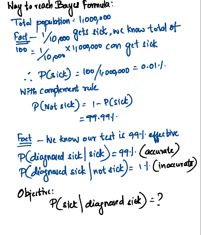
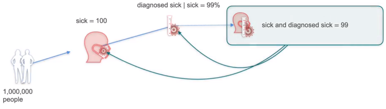
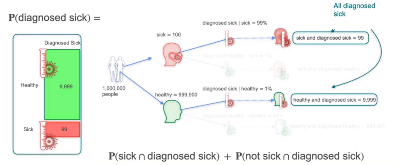
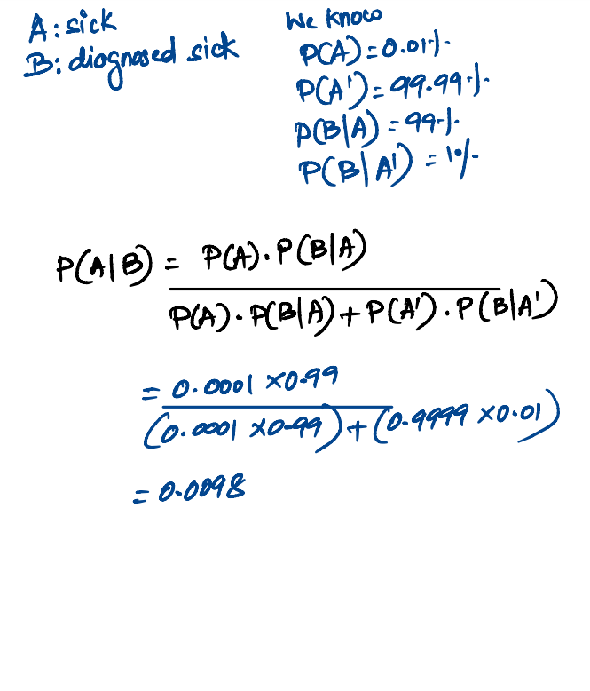
• Let’s say there’s a million people in the population, and let’s say that the illness only affects one of every 10,000 people. Now, the test that the doctor gives you is 99% effective. What does that mean? That means two things that out of every 100 sick people, 99 get correctly diagnosed as sick, and one gets incorrectly diagnosed as healthy. And among every 100 healthy people, one gets misdiagnosed as sick and 99 get correctly diagnosed as healthy.

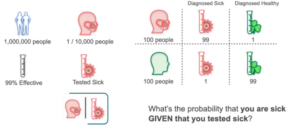
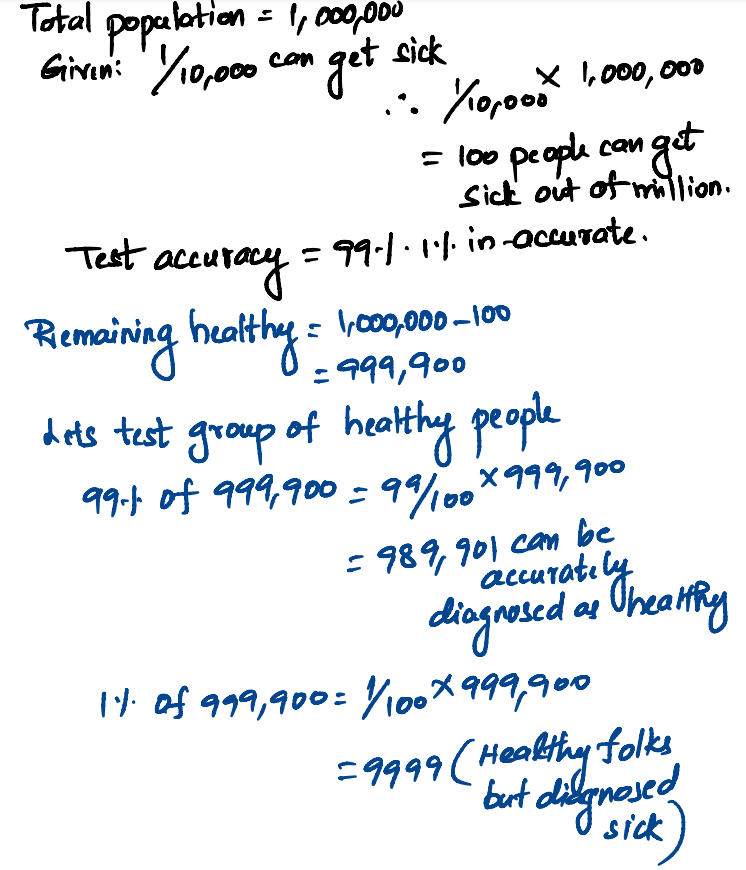
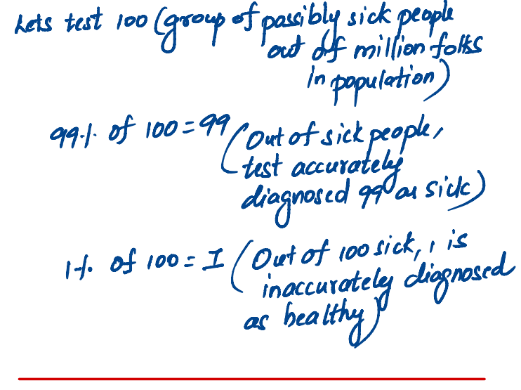
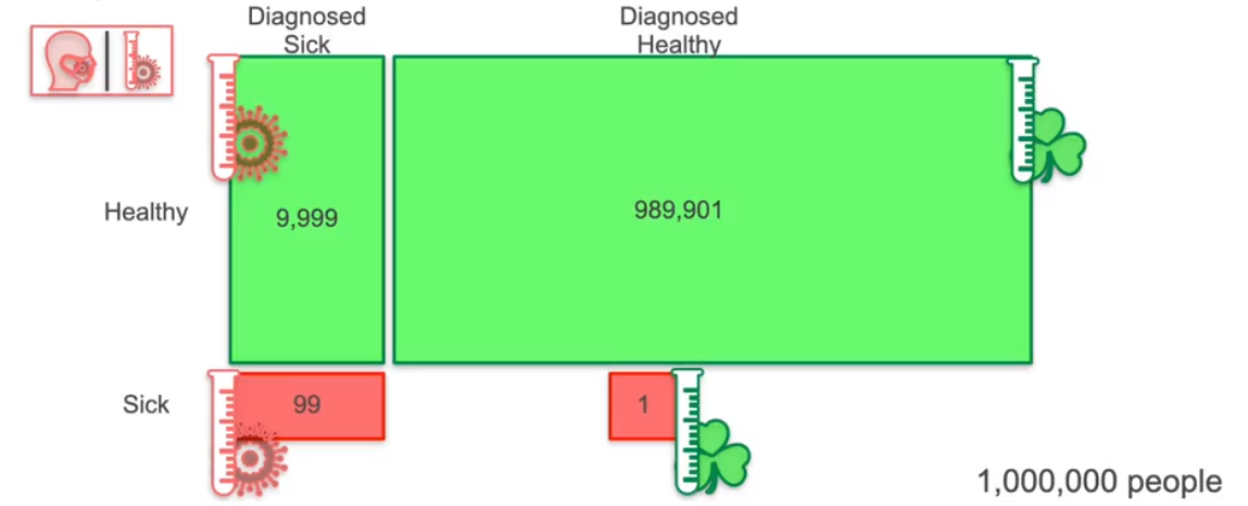
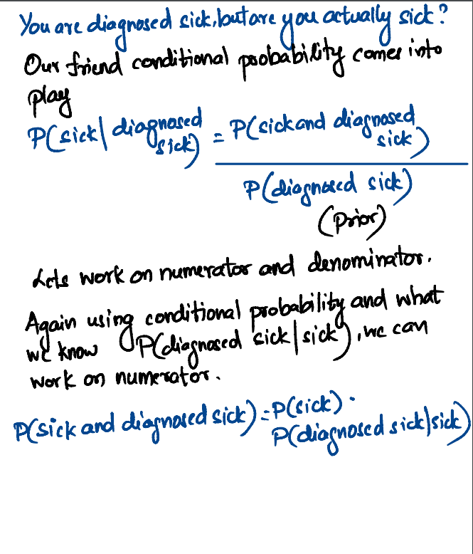
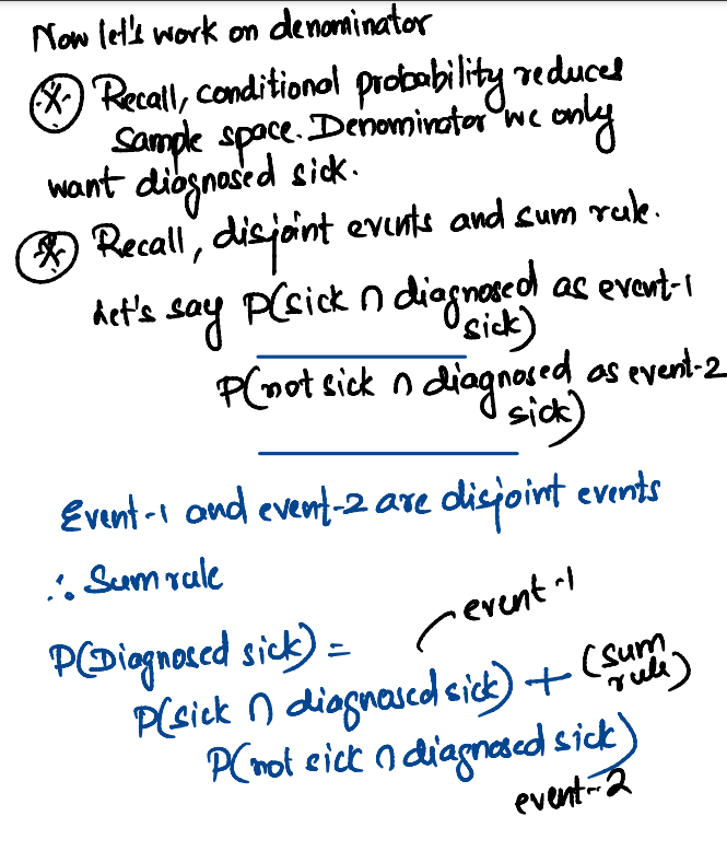
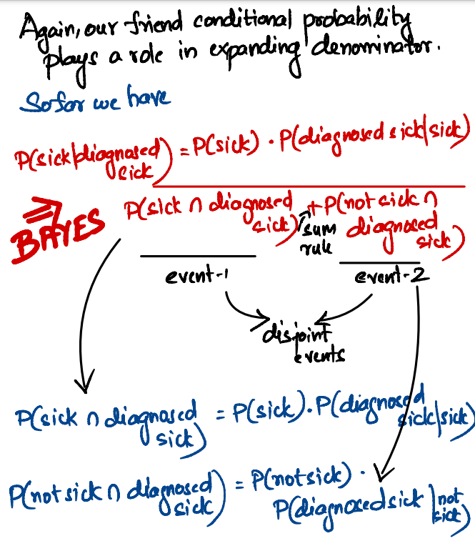
| Our friend conditional probability P (sick | Diagnosed sick) reduces the sample space only to include folks who are diagnosed sick

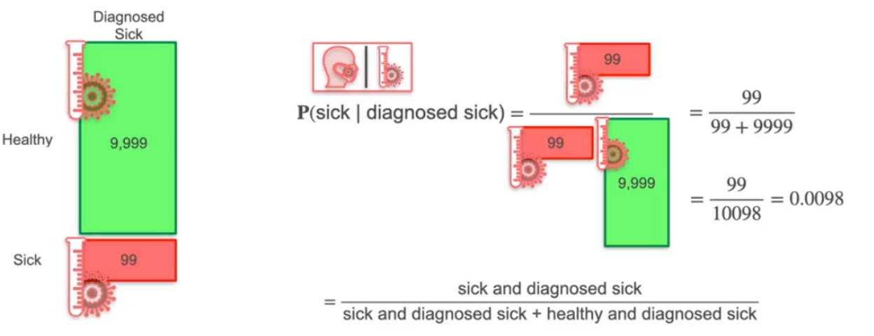
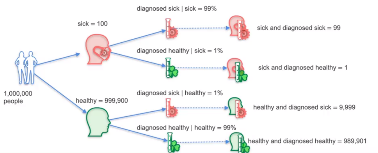
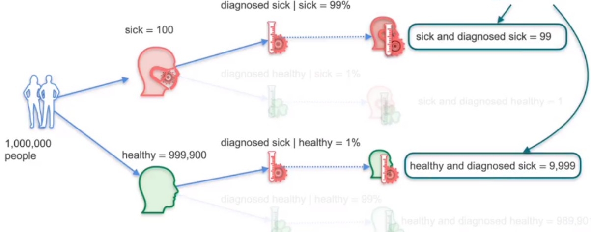
#Bayes formula - highlights

This section shows a way to reach Bayes formula and again we reach the same result of 0.0098 probabilty of being sick when you know that you are diagnosed sick.

#Naive Bayes model

In this post, I will share highlights of classic spam/ham example using Bayes theorem and making naive assumptions

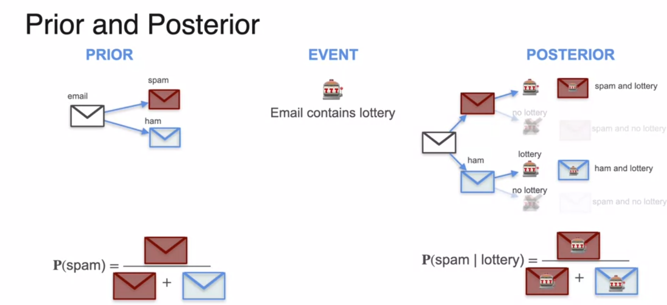
• By using Bayes formula which in turn depends on conditional probability, we are again reducing the sample space to only emails or text containing the words which we care about like “lottery”, “gift” etc.
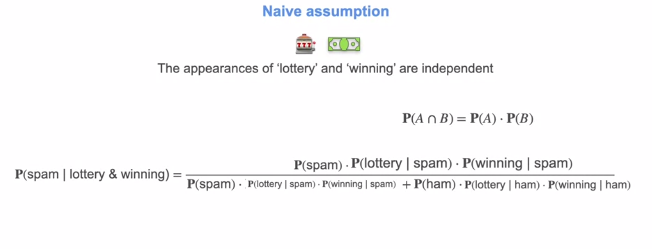
• Recall, the point from above on importance of independent events. If events are actually independent or if we can assume events are independent, then it makes our life easy. In few moments, let us see naive assumption we make.

Formalizing now

Prior => the original probability that you can calculate, not knowing anything else. Event => The event gives you information about the probability Posterior => With that information, you can calculate something called the posterior.

| The posterior is always a better estimation than the prior because we have that event that gave us information

In the following you can also see the reduce sample space, thanks to our friend conditional probability again.

#Naive Bayes Model

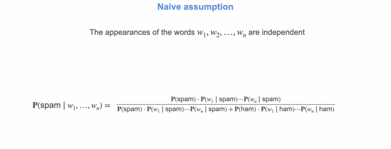
The crux of the model is naive assumption. With our classic spam,ham example above, let us say if there are other words we like to consider. For n words, assuming those n words do not appear together or in othre words independent makes calculation easy with just product.

#Random Variables

It is important to understand the following path. Events => random variable => probability distributions which can be for discrete or continous random variables (probability mass function vs probability density functions).

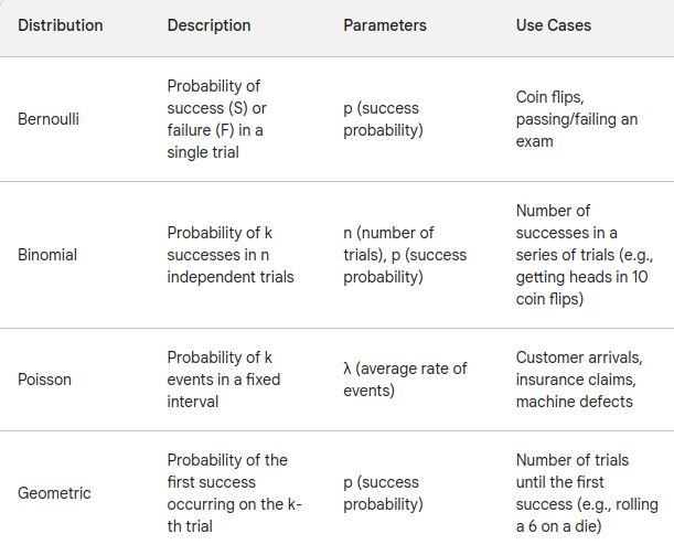
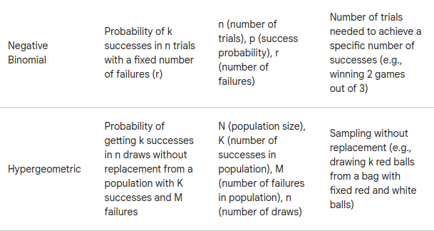
Probability distributions can be extended to multiple variables. It is important to understand the importance of co-variance in understanding the combined effect of multiple variables. I am not going to go deep. I have requested Google Gemini to create a cheat sheet of commonly used probability distribution and here we have

#Discrete Distributions

#Continous Distributions

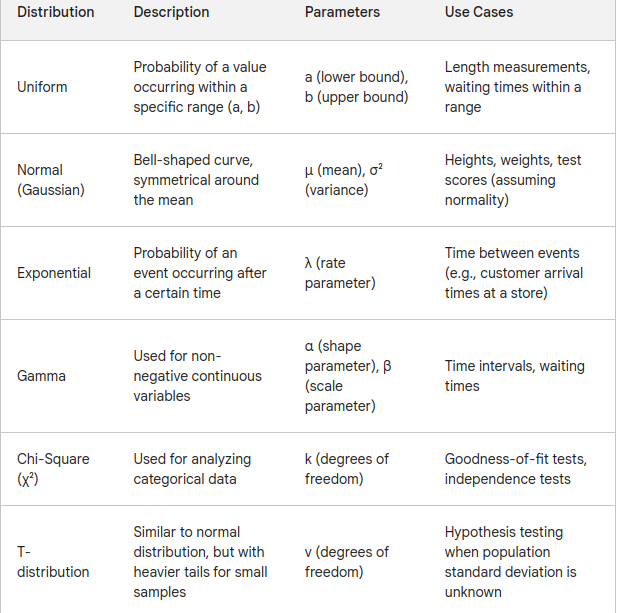
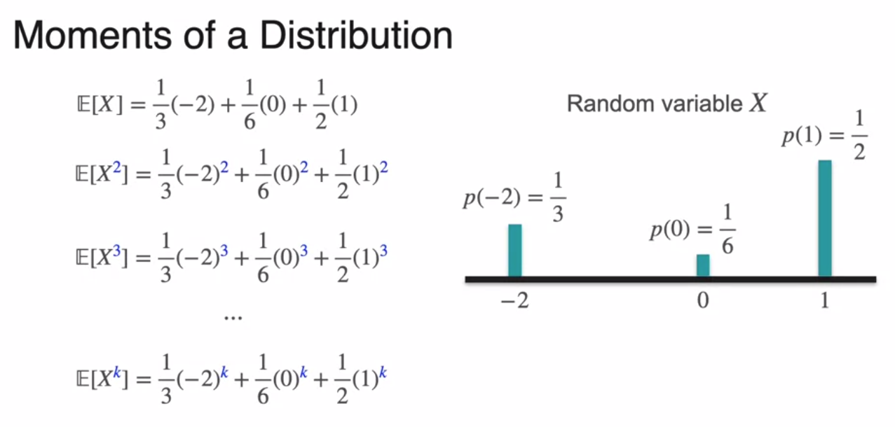
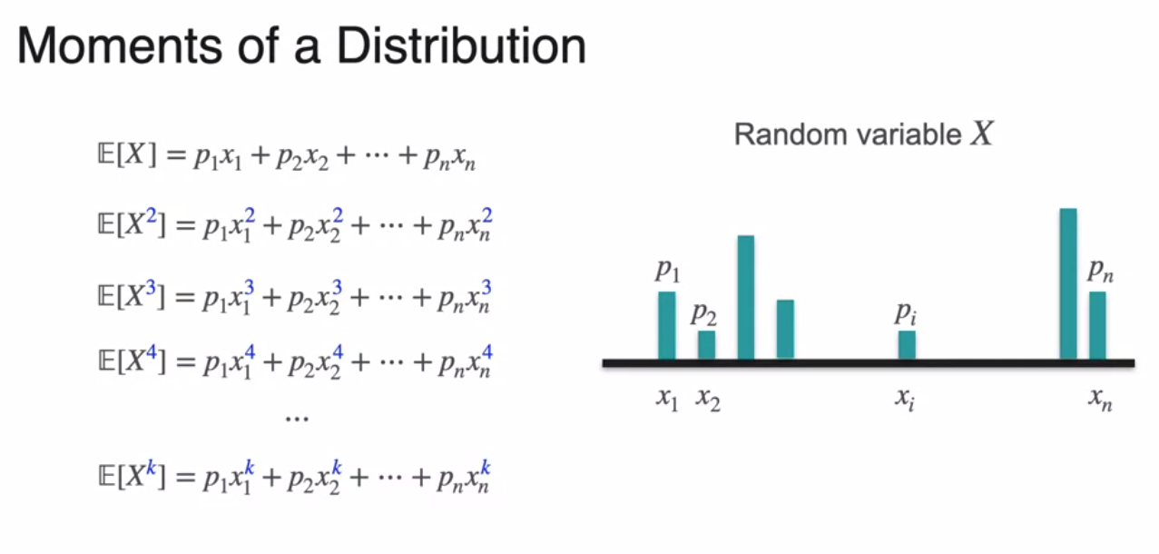
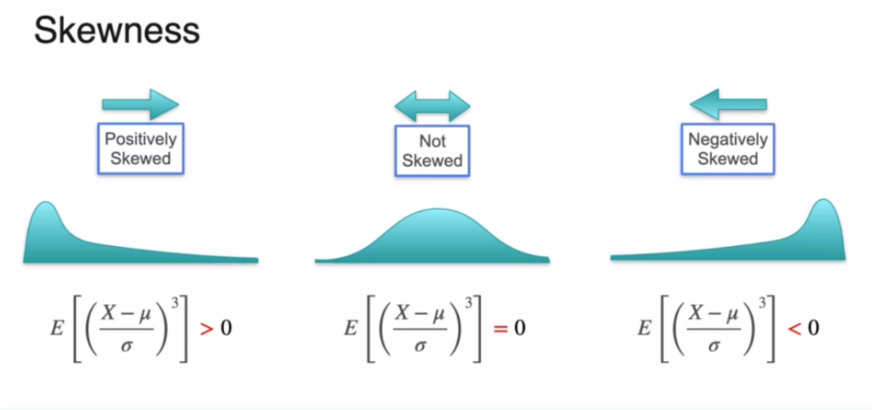
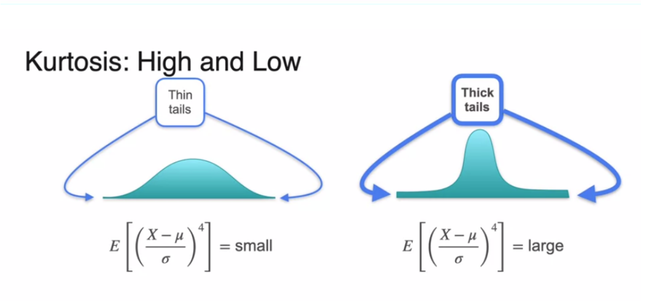
Next, I like to highlight about several ways to tell distributions are apart. Lets call it as moments of distribution. First moment as expected value, second moment (variance), third moment standardized (skewness), fourth moment standardized (kurtosis).

In general, if the random variable can take the values x_1 up to x_n with probabilities p_1 up to p_n, then the first moment is sum of p_i x_i the expected value. The second moment is sum of p_i x_i squared. Third moment is sum of p_i x_i cubed. The fourth moment is sum of p_i, x_i to the forth and so on until the kth moment, which is sum of p_i x_i to the k

#Visualizations

The post won’t be complete without touching upon few of my favorite visualizations and necessary topics.

Here is the flow to understand and remember following

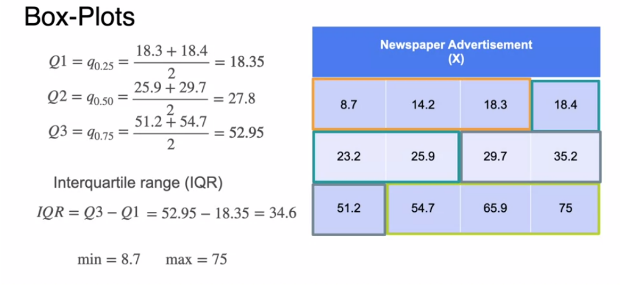
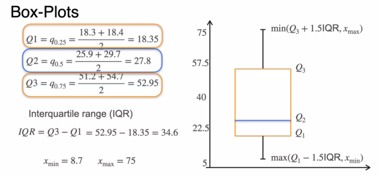
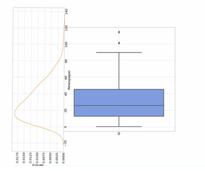
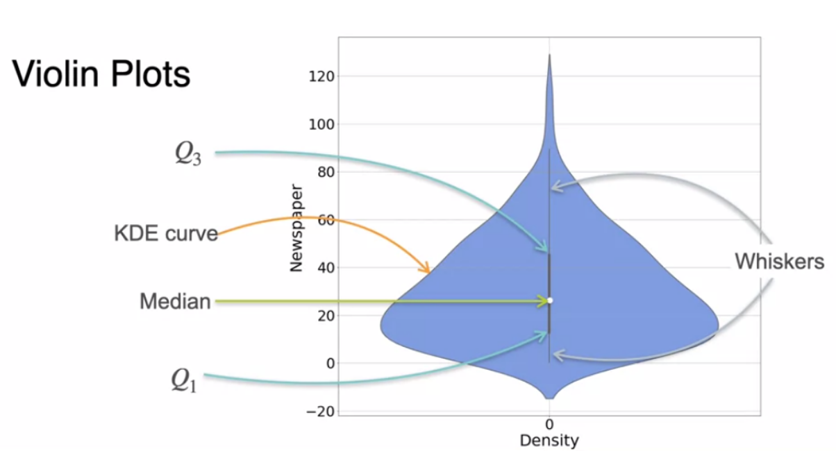
Quantiles => Box-Plots (25% quantile (1st quartile), 50% quantile, 75% quantile, min and max), Histograms => Kernel Density Estimation => Violin Plots

To save space for my favorite next topic where we will touch upon calculus relationship and view the relationship between likelihood, regularization and square error (regression - fitting line to data); I like to keep this section of notes short.

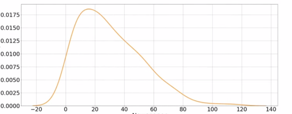
Next, PDF (Probability distribution function) of continous random variable can be visualized using Histogram. PDFs are usually a smooth function and also the discontinuities of the bars appear from the technique used to compute histograms and not from the data itself. This is where kernel density function comes into picture for better visualization of smooth distribution of continous random variable.

Below is kernel density estimation approximated view of continous random variable which is smoother than histogram.

Next comes Violin plot => Kernel density estimation + Box Plot

#Maximum Likelihood (my favorite topic) connects calculus (optimizing) + gives a reverse view of machine learning

GOAL - to share relevant math and notes related to likelihood, maximizing likelihood which in turn is optimizing a function in a similar way I have shown in my calculus post. In my opinion, maximum likelihood gives a different view (I usually call reverse view) of finding the best model which would have generated the data. Forward way can be fitting a model to a data and optimizing loss functions (refer to my calculus notes post). I will finish this post with Baysian inference sharing my notes related to regularization, squared error, maximum likelihood.

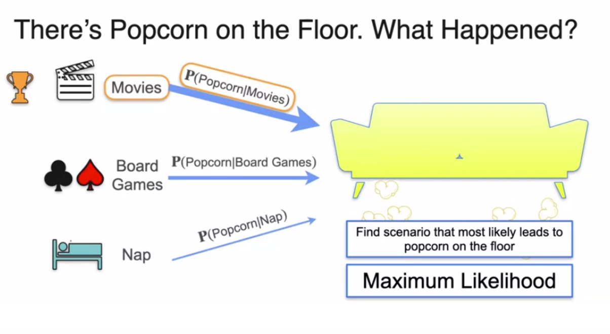
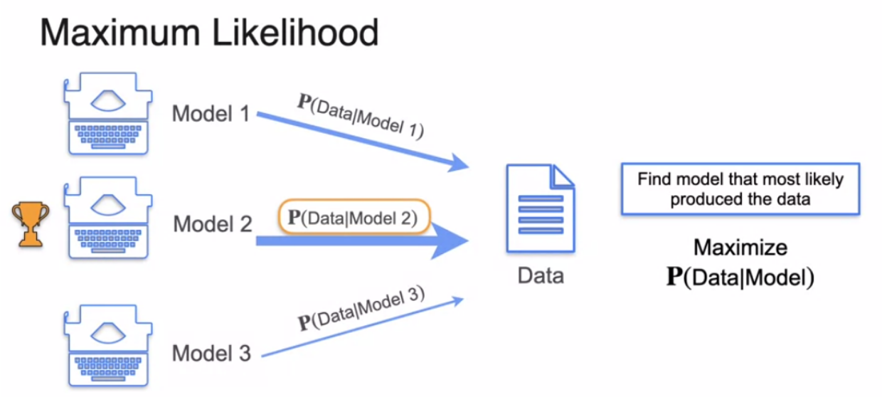
Let me begin with the famous analogy and explanation given by the best teacher Lois Serrano about maximum likelihood and let us see what I called as reverse view.

• Imagine that you have some evidence of something and you want to find the scenario that may have led to that evidence so you pick out of all the possible scenarios, the one that created the evidence with the highest probability.
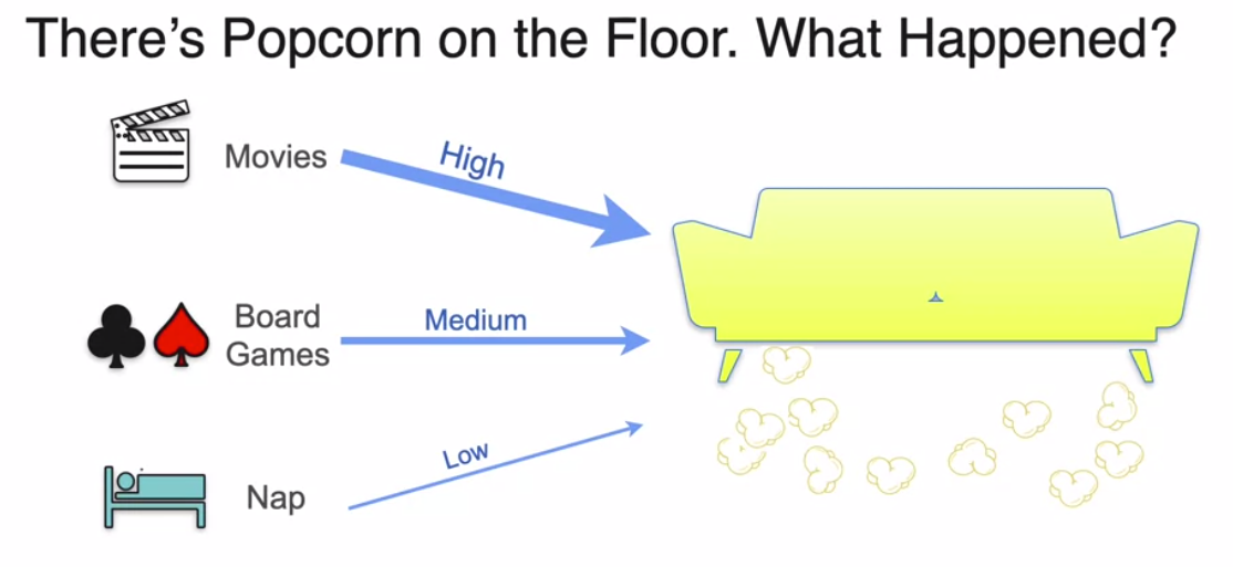
• Imagine that you walk into a living room and you see a bunch of popcorn lying on the floor next to the couch. Here’s a question for you. Which one of these events is more likely to have happened? People watching a movie, people playing board games, or somebody taking a nap. Which one do you think was more likely to have happened?

Now, the following gives a different view (in my words reverse view) of model fitting to data.

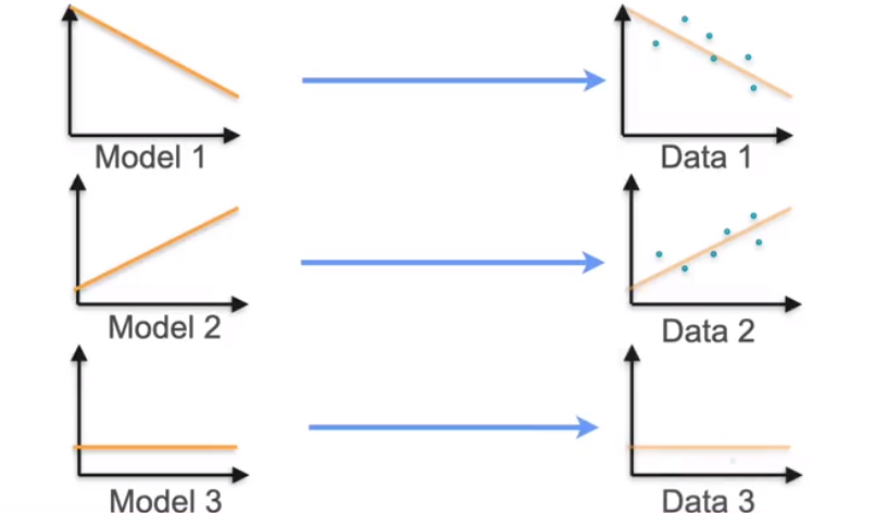
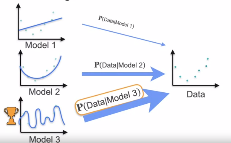
• You have a bunch of data and several models that could have generated that data. What you do is you estimate the probability that we see this data given Model 1. The probability that we see this data given Model 2 and given Model 3 and whichever gives the highest probability is the model that we pick, the model that most likely produced the data. In other words, we’re maximizing probability of data given model.

#Role of calculus + view of optimizing a function using Bernoulli distribution

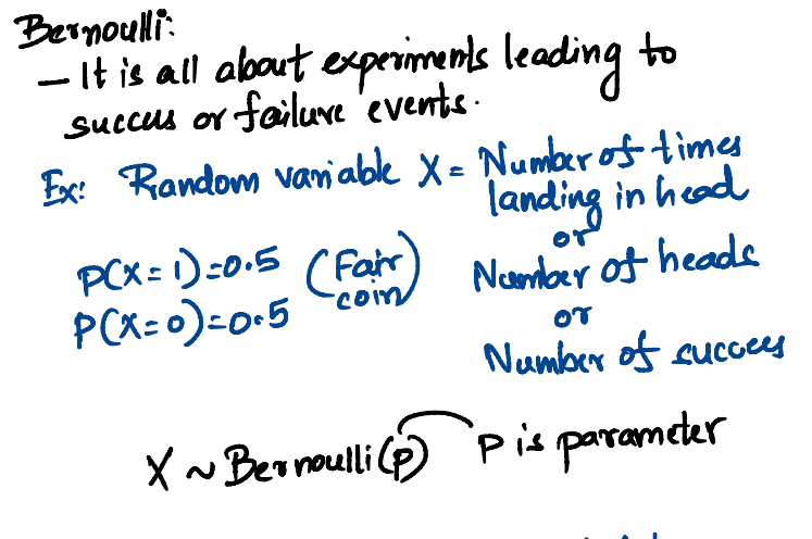
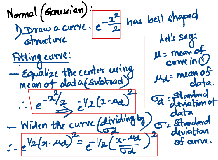
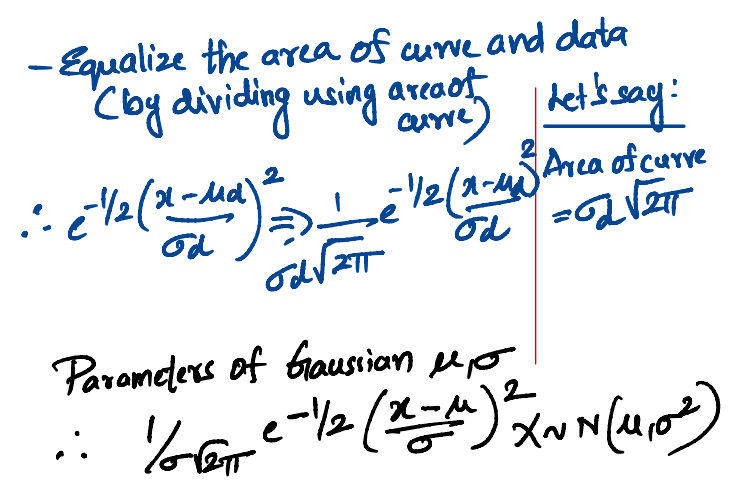
Before we look into likelihood of Bernoulli and maximizing them, I like to add a quick refresher on Bernoulli distribution and inevitable Gaussian distribution formula derivation.

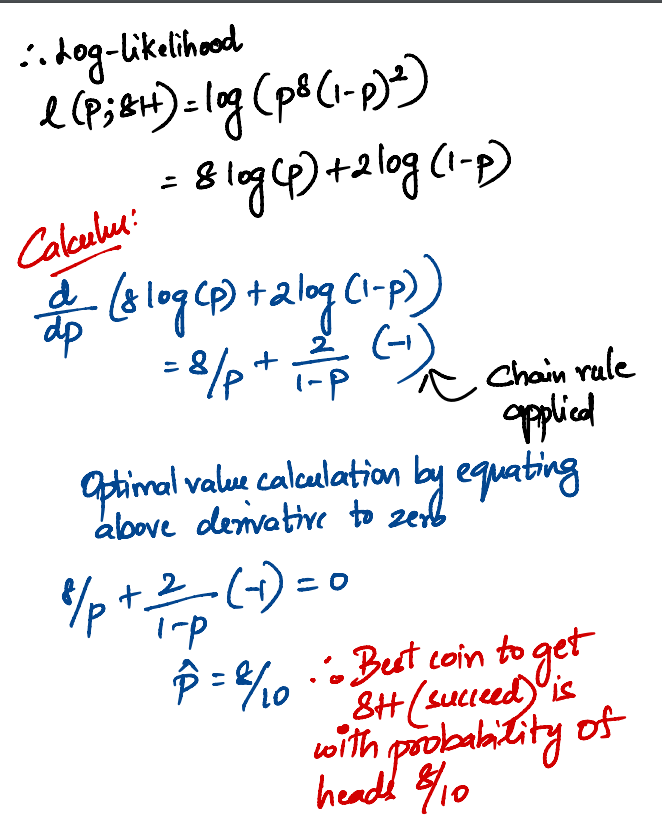
• Suppose that you toss a coin ten times and it lands in heads eight times and in tails twice. Now you have three possible coins that you could have flipped to get these results. Coin one has a probability of heads of 0.7, coin two is a fair coin, has a probability of heads and tails of 0.5 and coin three has a probability of heads of 0.3. Now, which one do you think was the coin used for these 10 tosses? Or at least which one would you use if you were aiming to generate those 10 tosses again?

In the above data can be result of tossing a coin 10 times => 8H2T (eight heads, two tails) and you can say that different coins are different models. Like I said before, in reverse, we will find the best model (coin) which has high likelihood to generate the data (8H2T)

We can also see analytically, without maximum likelihood estimation that coin one has highest probability.

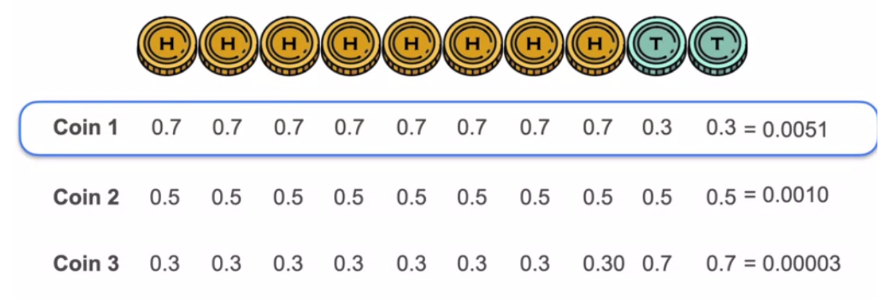
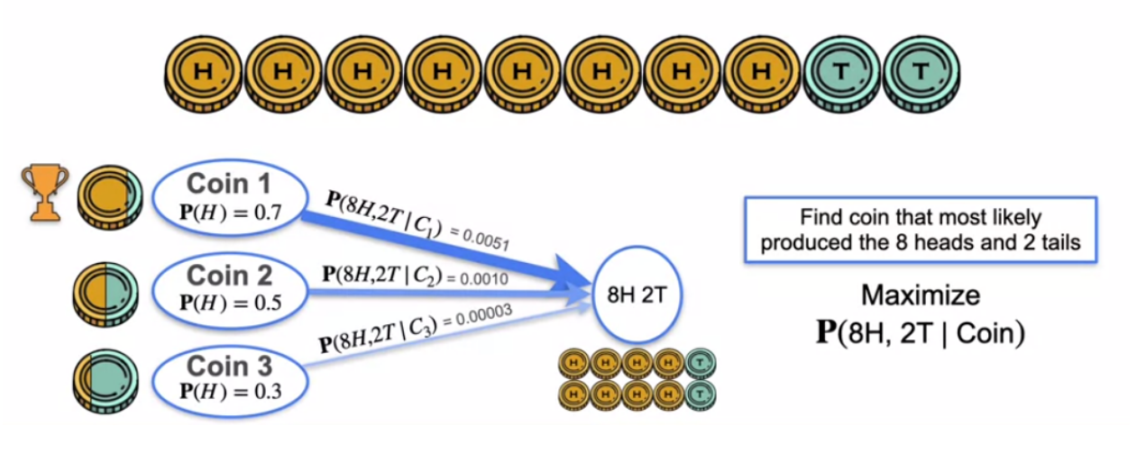
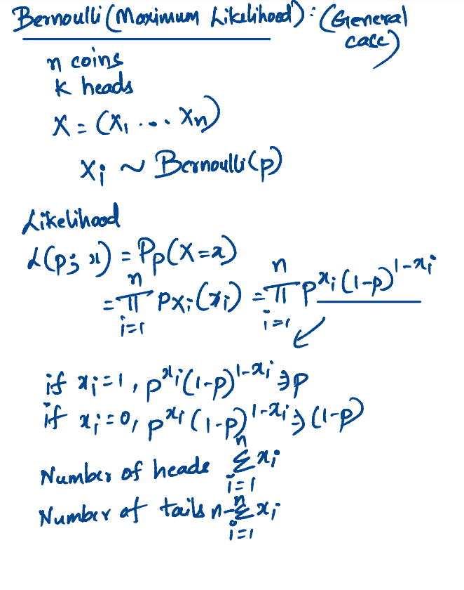
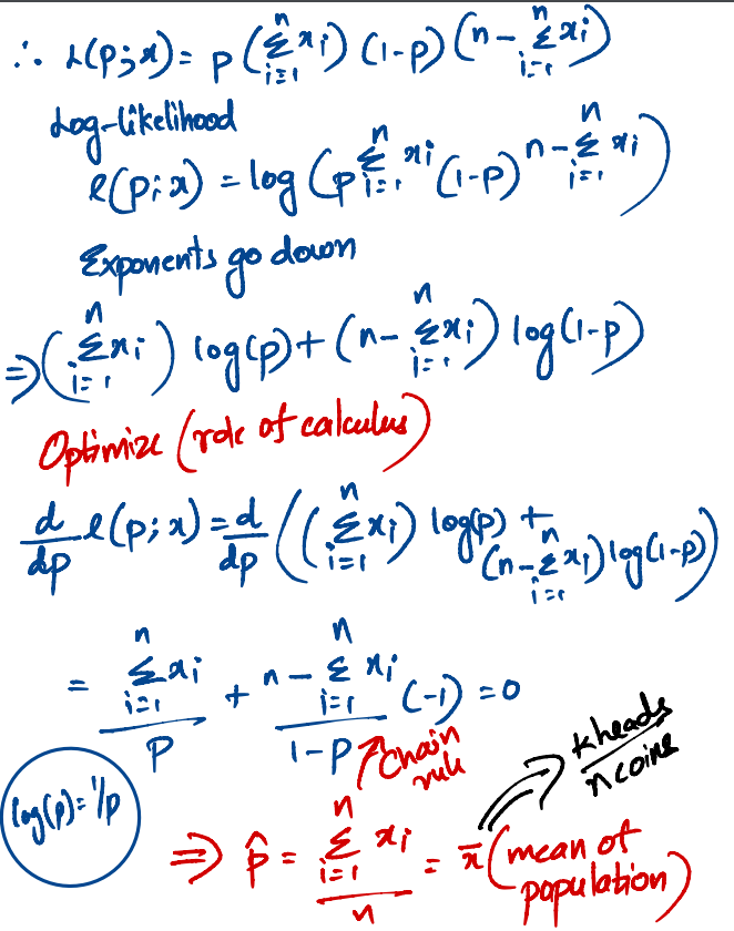
Now let us look into official maximum likelihood estimation of Bernoulli. My goal is to share my notes related to viewing the below as function of parameter which we want to optimize using calculus optimization techniques to find the best parameter which could possibly give us the result.

• Here is the flow likelihood => log-likelihood (to convert products to sum) => calculus derivatives and equating to zero => optimal parameters

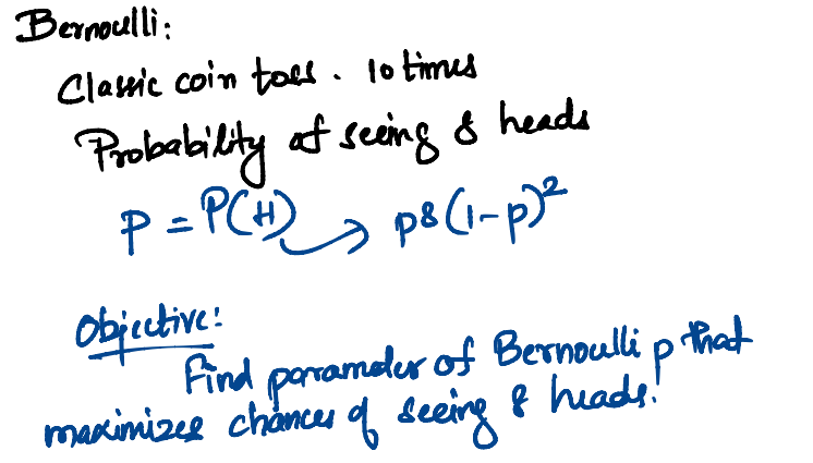
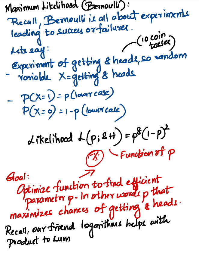
The above analytical conculsion matches with maximum likelihood estimation calculation showing the winner as first coin (which is biased)

Above concepts also applies to finding the optimal parameters (mu and sigma) of different Gaussian distribution which most likely generated the data or produced the result or produced the evidence (however you want to call it).

Let us go back to reverse view of finding the maxlimum likelihood candidate among different models which would have generated the data. Lets use a simple linear regression as example and look at the probabilistic (reverse view in my words) of finding the best model, rather than fitting a line to the data.

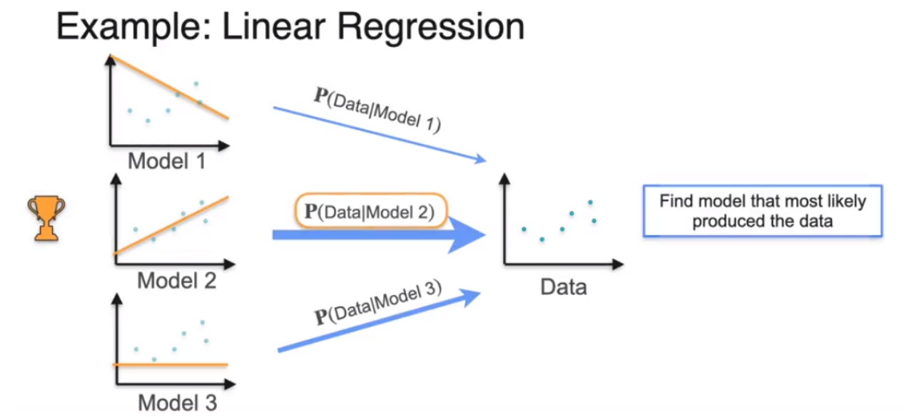
#Line to dots(data) - reverse view

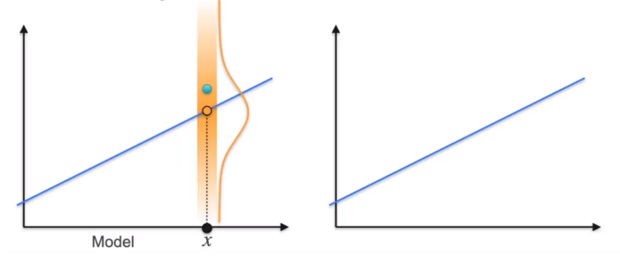
• Best analogy and exaplanation again by Lois Serrano. Imagine it as a road. If you have that road being the yellow line and you start building houses, the houses are likely to be built close to the road and not far from it.

You’re going to generate a point close to the line using a Gaussian. We put a Gaussian, and we center it at the point where the line meets the horizontal line. We’re going to sample out of that Gaussian, so we sample this one over here. That’s the same as saying, we’re going to build a house that is likely to be close to the road and it’s going to be sampled from vertical Gaussian.

If we have a bunch of points x_1 up to x_5, then we have five Gaussians all centered at the point on the blue line. From each one of these, we’re going to sample some point. Below shown are the five points that we’re sampling based on this blue line.

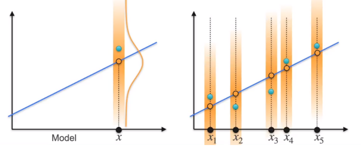
| Summary - Line that best produced the points == Line that best fits the data(linear regression)

• Let’s say that the line has equation y = mx+b, and there are the points of intersection with the line and there are the generated points.
• The distances are going to be called d_1, d_2, d_3, d_4, and d_5.
• First, let’s calculate the likelihood of generating this point. Since we have a Gaussian, then what really happens is that the Gaussian is centered at the point where x_1 intersects that blue line.
• If we assume that it’s a Gaussian with standard deviation one and mean equal 0, then the likelihood of generating these point is given by the formula of the Gaussian which I derived and showed above. It will be the Likelihood of generating the first point.
• We’re looking at all of them. That’s the product of the five likelihoods. That’s what we have to maximize.
• We have to maximize the likelihood of the line generating all those points. Since they’re independent, then we have to look at the product.

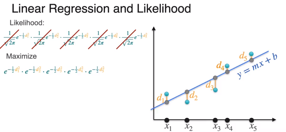
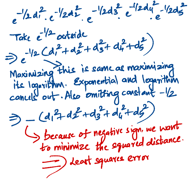
In linear regression, you want to find the blue line that minimizes the sum of squared distances from the point. This shows that finding the line that most likely produce a point using maximum likelihood is exactly the same as minimizing the least square error using linear regression.

#Regularization (recap)

#Bayesics

Conditional probability comes into picture. Baysian way of including the prior and yet another interesting analogy used by Lois Serrano is interesting concept which cannot be missed in this post.

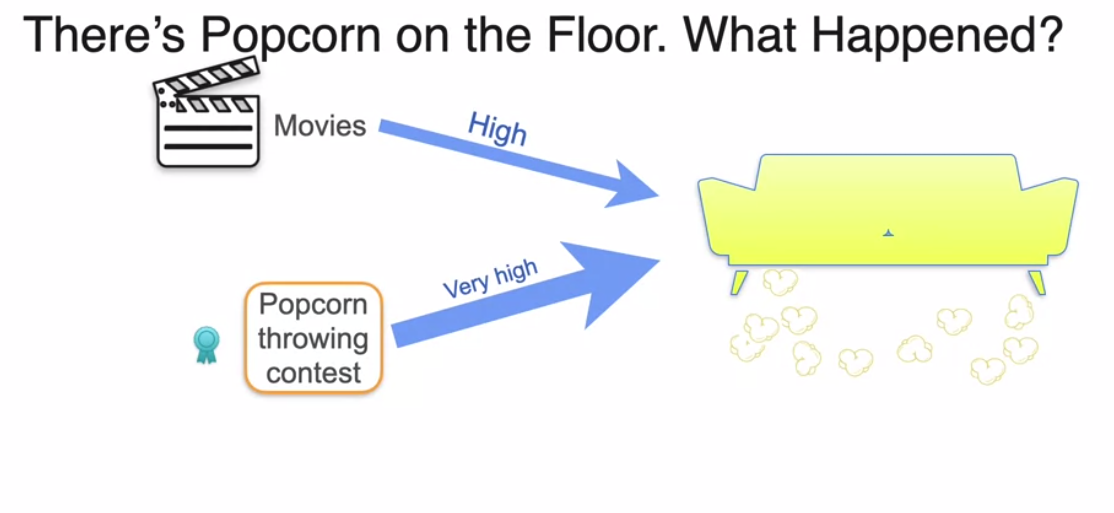
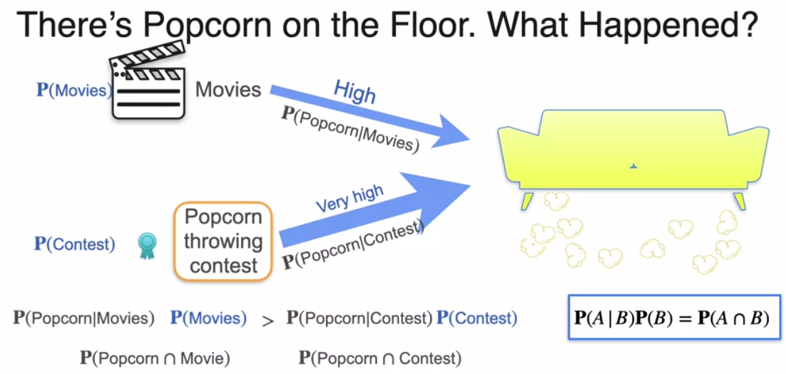
• So let’s go back to our example where we had some evidence which was popcorn in the floor and three possible scenarios. And we’re trying to investigate which scenario happened. The first one is movies, which creates the popcorn with a high probability. The second one is board games, which creates popcorn with a medium probability. And the third one is a nap that creates popcorn with a very low probability. So we went for movies, which is the one that generated the evidence with the highest probability.
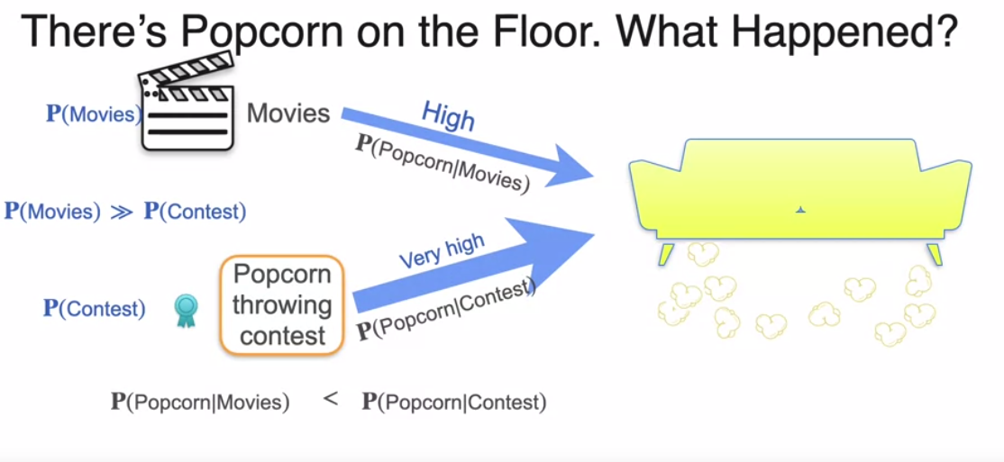
• Imagine that now we have two different candidates. One is that we were watching movies, and the other one that there was a popcorn throwing contest. So movies create popcorn in the floor with high probability, but a popcorn throwing contest would create popcorn in the floor with a very, very, very high probability. It’s almost for sure that if you have a popcorn throwing contest, that you ended up with popcorn in the floor. So that’s the winner. However, something tells us that movies should be the winner and not popcorn, why? Well, one reason is that it’s likely that you could have been watching movies. A popcorn throwing contest is not very likely. It’s a very unlikely event. So even though it’s more likely to have generated the evidence, it’s less likely to have happened on its own, and that should matter.

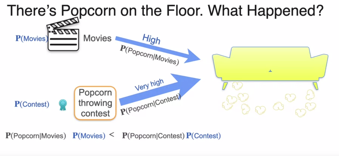
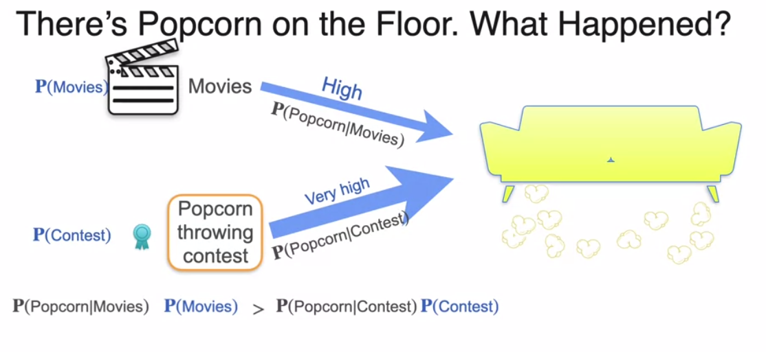
• Before what we did is maximize the probability P(popcorn/scenario). So we figure out that P(popcorn/movies) was higher than P(popcorn/contest). However, the probability that you’re watching a movie by itself is actually higher than the probability that there was a popcorn contest. It’s actually much higher. And so we should factor this into the equation. So we should actually multiply them. And when we have the product, then the inequality goes in the other direction.

Our old friend conditional probability comes into picture again

• Therefore, we’re trying to maximize the probability that there’s popcorn and a movie and the probability that there’s popcorn and a contest. That’s really what we care about in maximizing both.

• Let’s say you have the data and you have three models that could have fit that data, and each one of them generates the data with some probability and remember that a model can generate the data as we saw before by simply creating a Gaussian at every point on the line and generating points close to a line or to the curve.

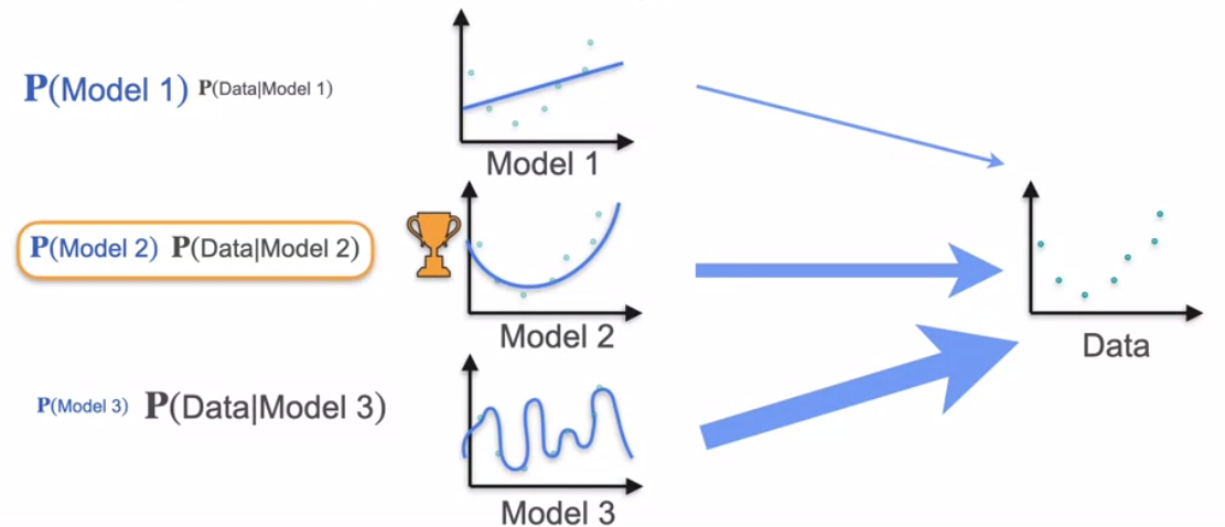
Now with Baysian mindset, if we also include individual probabilities of the model itself

• we’re going to do, is we’re going to multiply these probabilities and now the winners, not the third one. Now perhaps the winner is the second one and so this is the winning model.

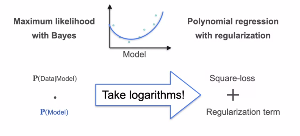
• In regression we are going to have some loss that can be the square loss(example), and in maximum likelihood you’re going to maximize the probability that the data was created with the model.

• With Bayes, we will multiply with probability of model

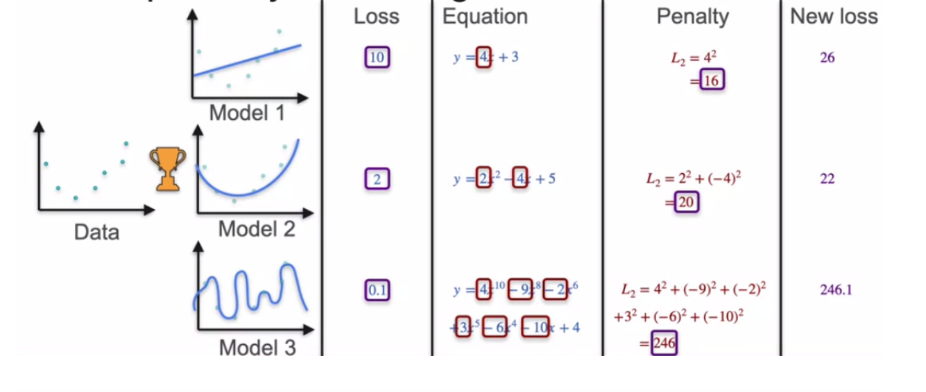
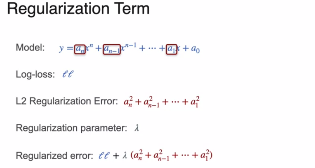
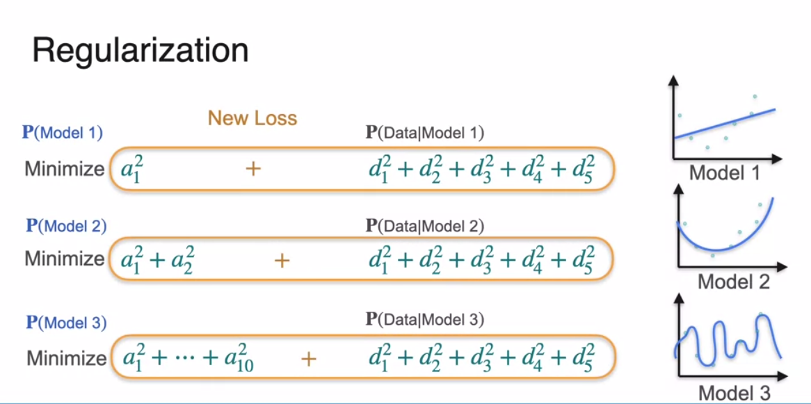
• With Square loss, we add regularization term to avoid overfitting

• Let’s say we have Model 1, Model 2, and Model 3 and there’s a high probability for Model 1, a small one for Model 2, and really small one for Model 3. Well, let’s say that these are the equations for the models. What we’re going to do is we’re going to pick these coefficients out of a standard normal distribution, so a_1, a_2 and all those up to a_10, are going to be selected from a standard normal distribution.

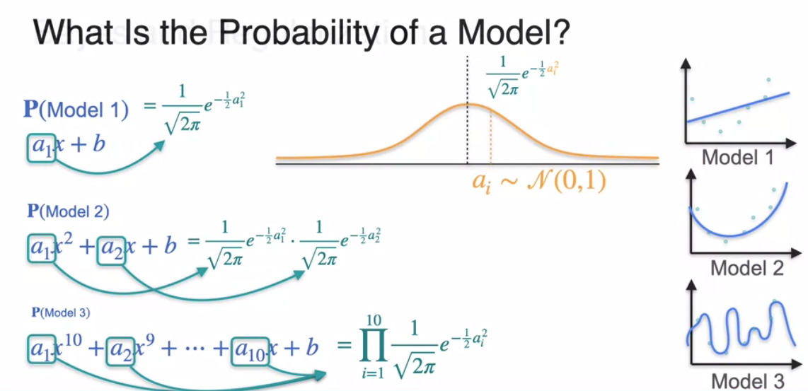
Refer to the explanation above on square loss minimization is equal to finding maximum likelihood

Now in a similar way and with Baysian hat, let us include probability of model itself with maximum likelihood. Now if we solve algebrically like above, we will be minimizing nothing but square loss and extra regularization terms included which comes from the probability of the model we included

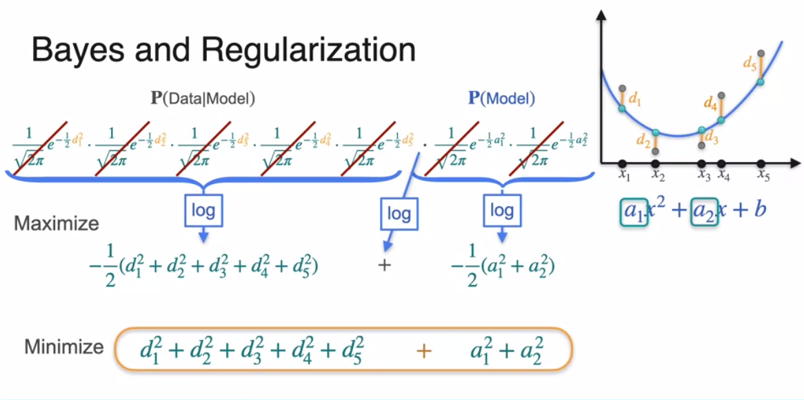
Therefore, when we try to pick the model out of Model 1, Model 2, and Model 3, then maximizing the probability of a model is the same as minimizing the sum of squares of the coefficients and maximizing the conditional probability of the data given the model is the same as minimizing the square loss. The new loss is going to be the sum of the two and that is how you train a model using regularization based on Bayesian approach.

#Conclusion

This post is a tribute to wonderful teacher and mathematician, my favorite Lois Serrano. I have written this post in a way to highlight the topics which covered my interest. I am sure there are lots of other interesting topics. Remember the importance of conditional probability and also the reverse way or probabilistic way of viewing machine learning. I thoroughly enjoyed writing this post. I hope it helps someone else too in addition to me.

#References

• Best teaching and words of Lois Serrano
• https://www.coursera.org/learn/machine-learning-probability-and-statistics
• Cheat sheet for probability distribution was a result of my question to https://gemini.google.com/.
• Except all handwritten notes, some of the images comes directly from course notes itself and if not, I should have added credite to source of the image.