Essence of Calculus, its role in machine learning

#Essence of Calculus Notes

• My goal is to share my notes related to Calculus in the context of Neural Networks, contrasing with Linear Algebra and best resources which helped me.
• This is part of #Yet_Another series where the topic is not brand new and many have written and shared their knowledge.
• Nevertheless, I also like to share my notes from several popular resources which are not limited to the following from which some of the below notes are captured.

• Mathematics for Machine learning specialization - Imperial College London
• Mathematics for Machine learning and Data Science Specialization - Coursera by my favorite Lois Serrano
• Best Book Mathematics For ML

#Non-Objective

• To write about calculus rules, formulas including famous chain rule.

#Objectives

• Following notes cover topics related to Jacobians, Hessian, Determinant of Jacobian, unconstrained optimization, touch upon constrained optimization, automatic differentiation which is greatly abstracted with modern deep learning frameworks like Pytorch, Tensorflow, Jax with their autograd, autodiff respectively. I also like to touch upon basic building block of neural network which is perceptron, multiple perceptrons and role of activation functions which sheds light on efficient non-linearity. Neural Network gains advantage with non-linearity introduced by the appropriate activation functions.

#Introduction

Above said courses, lot of books and resources covers famouse rate of change of speed with respect to time as a basic example to describe derivates. However, my favorite is geometric view of derivates.

(Difference Quotient). The difference quotient computes the slope of the secant line through two points on the graph of f. The difference quotient can also be considered the average slope of f between x and x + δx if we assume f to be a linear function. In the limit for δx → 0, we obtain the tangent of f at x, if f is differentiable. The tangent is then the derivative of f at x.

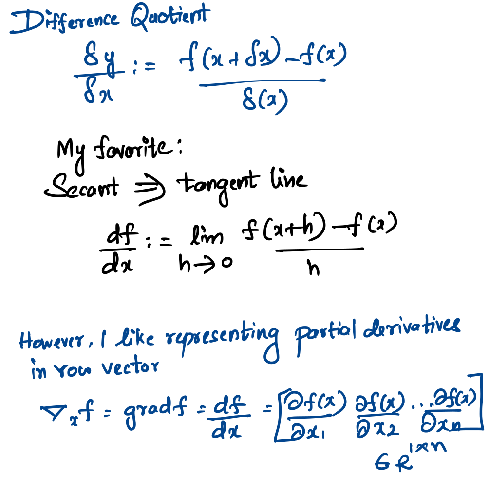
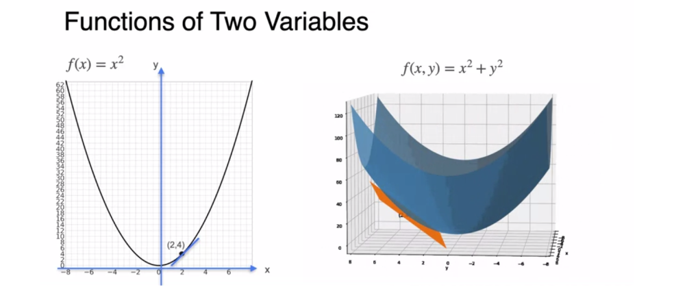
• Now the idea of secant becoming tangent line transforms to tangent plane when two variables plays the role which will be a good segway for partial derviates topics. Partial derivates leads to Jacobians and Hessians.
• I am not going to go deep on first order derivates, second order derivates and famouse sum, product, chain rules. However, you will see partial derivates used in this post.Its inevitable.

#Partial-Derivates [Gradients]

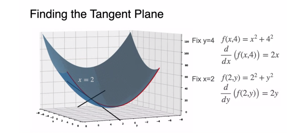
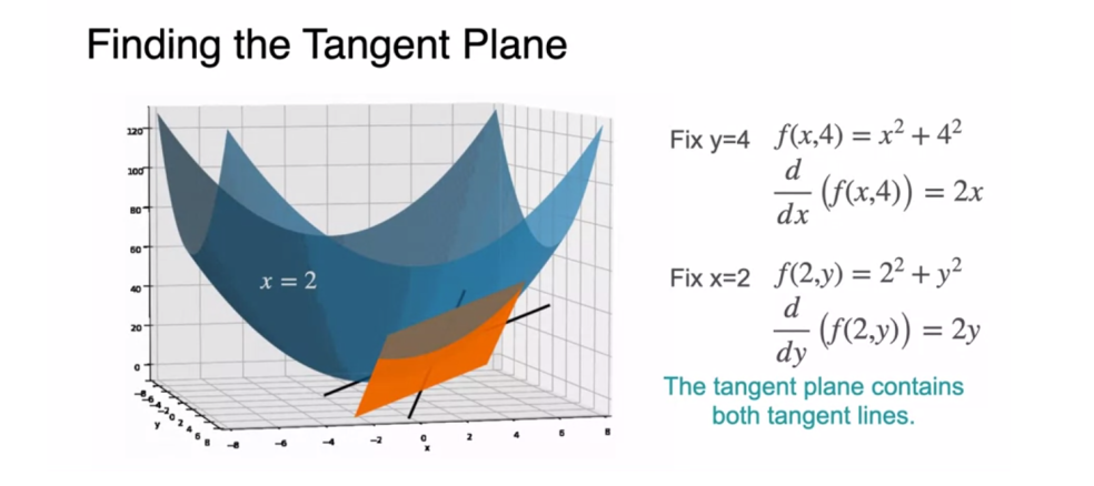
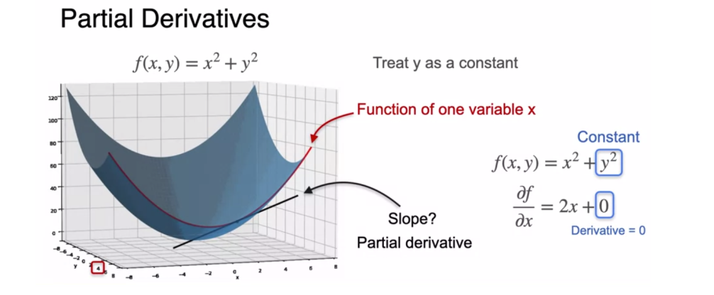
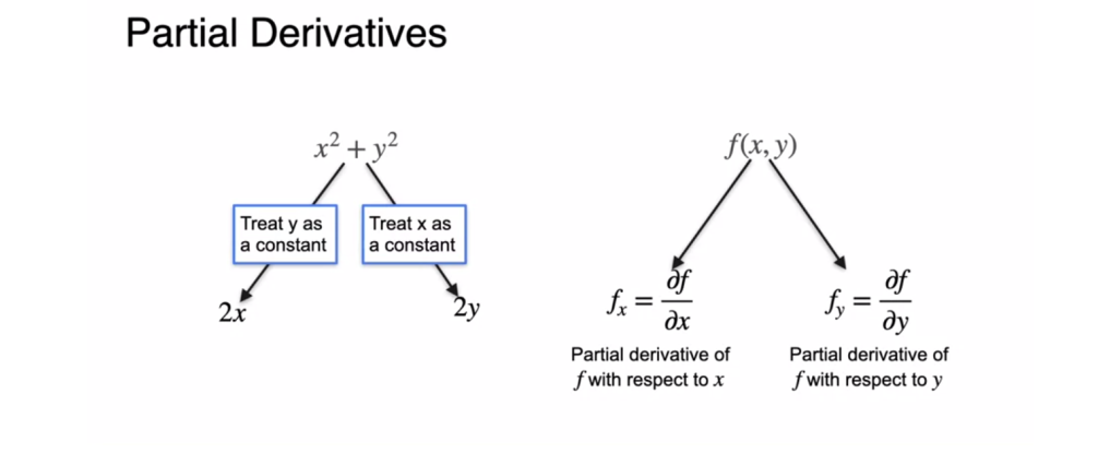
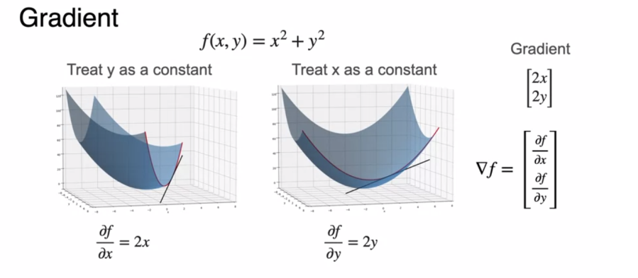
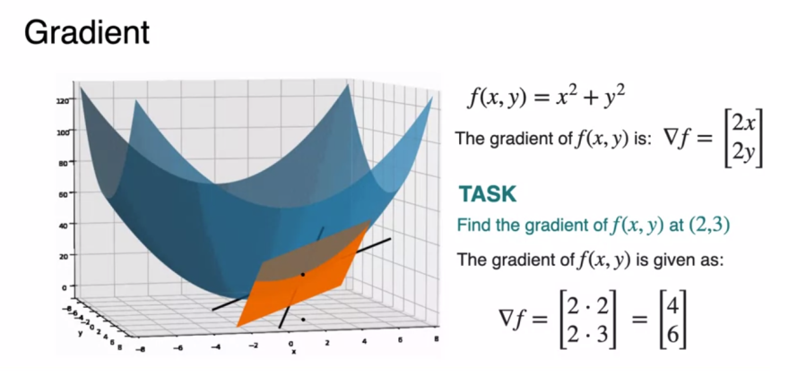
• Again, my favorite geometric view of partial derivates in the context of two variables, tangent plane and partial derivates acting as a slope. In a function of two variables, when you treat one as constant, then it becomes a function of one variable. Now as we saw in one dimension, we can draw a tangent line and partial derivative becomes the slope of the line.

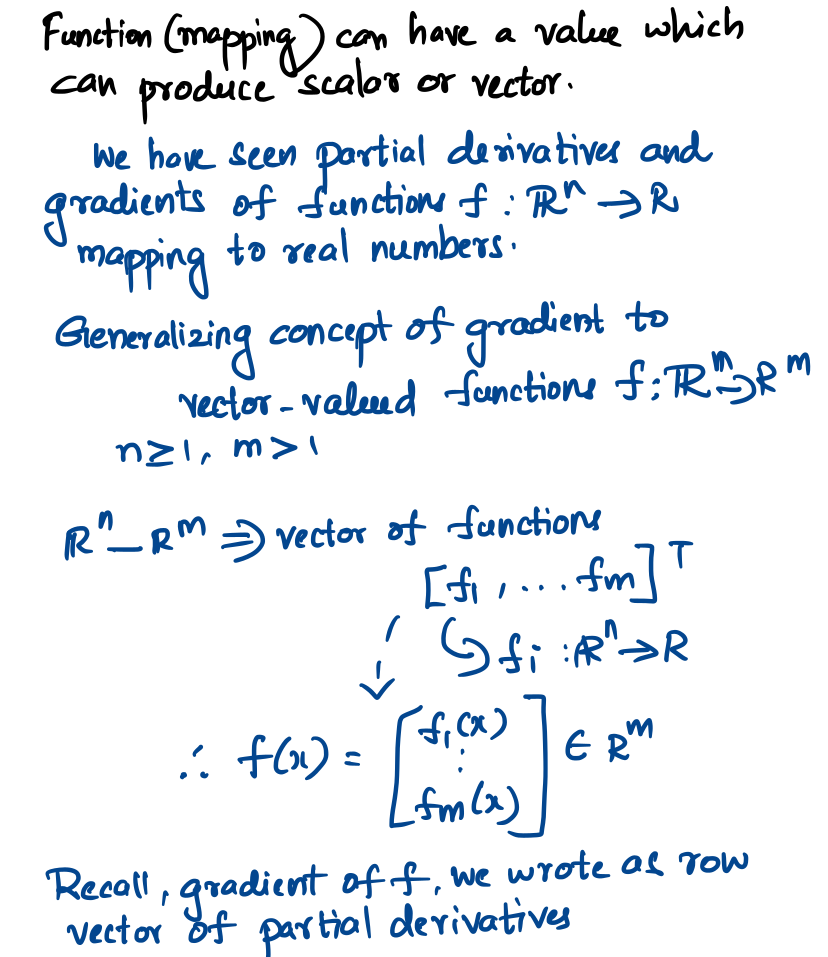
#Jacobians Matrix (Vector Valued Functions) in contrast to special case Jacobian Vector

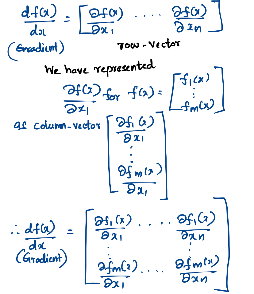
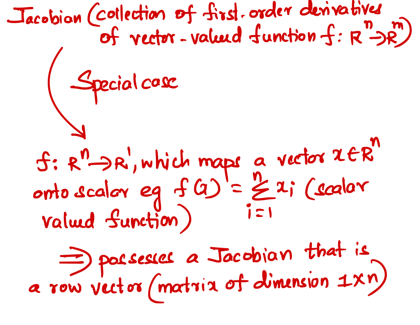
• My favorite topic from MML book above, which shows two approaches related to Linear-Algebra and Calculus. I also like to quote the dimensionality of partial derivates based on function mappings. Let us explore in this section the importance of Jacobian determinant, vector and Jacobian matrix product which leads to Autograd later. This is one of my favorite sections.

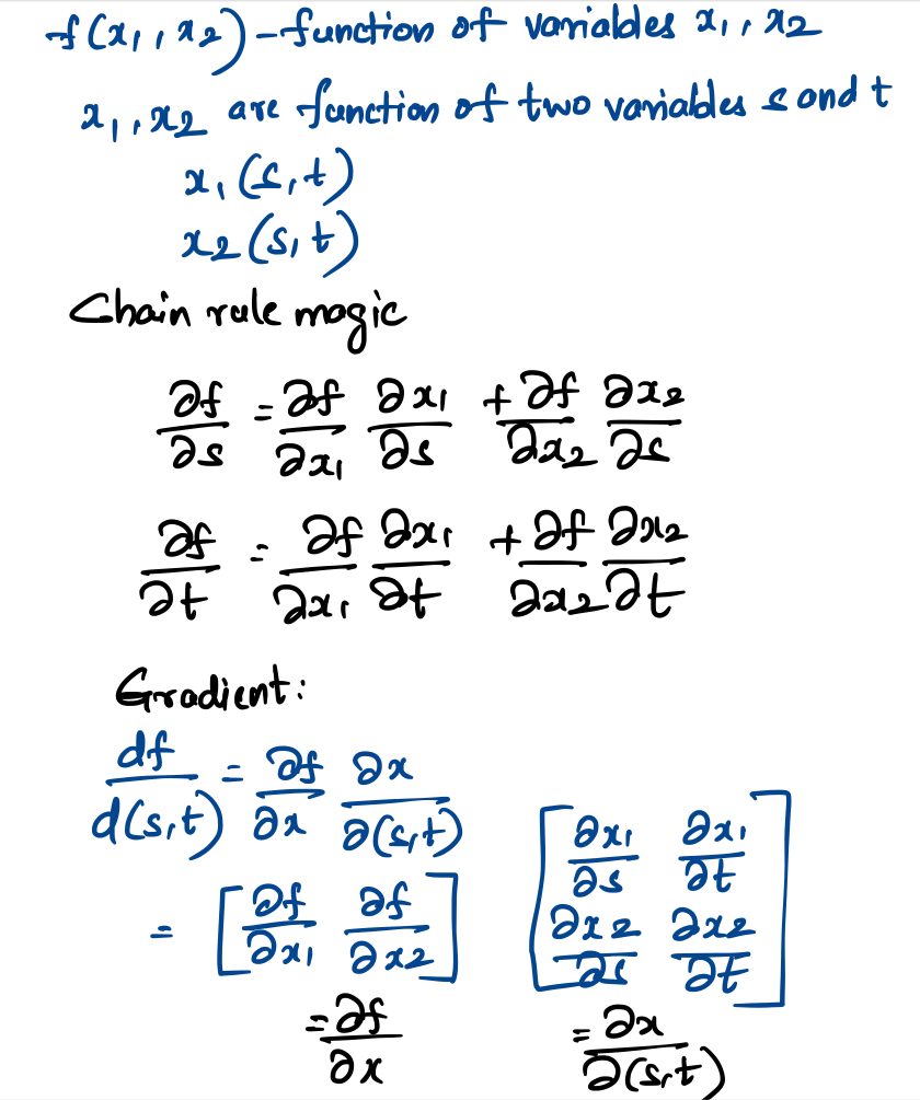
(Jacobian). The collection of all first-order partial derivatives of a vector-valued function f : Rn → Rm is called the Jacobian.

#Determinant of Jacobian Matrix

Change of basis, determinant concepts from Linear Algebra plays a role in finding the area and also transformation. I am not going to write about calculating determinant of matrix or change of basis. Please refer to the above cited book or online resources.

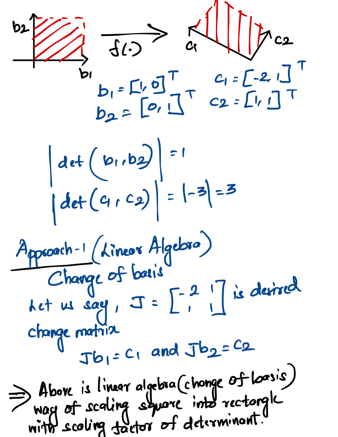
The area of scaled rectangle is exactly three times the area of the unit square. We can find this scaling factor by finding a mapping that transforms the unit square into the other square. In linear algebra terms, we effectively perform a variable transformation from (b1 , b2 ) to (c1 , c2 ). In our case, the mapping is linear and the absolute value of the determinant of this mapping gives us exactly the scaling factor we are looking for.

Calculus Approach

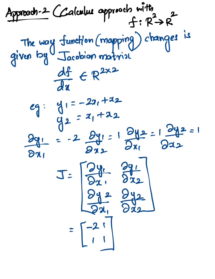
For this approach, we consider a function f : R2 → R2 that performs a variable transformation. In our example, f maps the coordinate representation of any vector x ∈ R2 with respect to (b1 , b2 ) onto the coordinate representation y ∈ R2 with respect to (c1 , c2 ). We want to identify the mapping so that we can compute how an area (or volume) changes when it is being transformed by f.

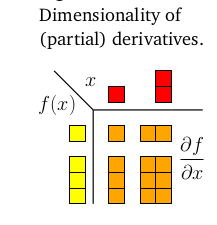
Another interesting from MML book which should be part of notes related to Calculus for deep, machine learning is following figure which summarizes the dimensions of those derivatives. If f : R → R the gradient is simply a scalar (top-left entry). For f : RD → R the gradient is a 1 × D row vector (top-right entry). For f : R → RE , the gradient is an E × 1 column vector, and for f : RD → RE the gradient is an E × D matrix.

#Perceptrons

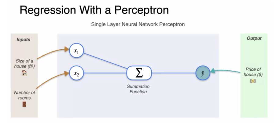
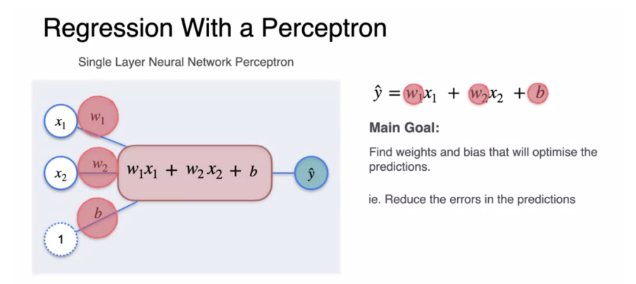
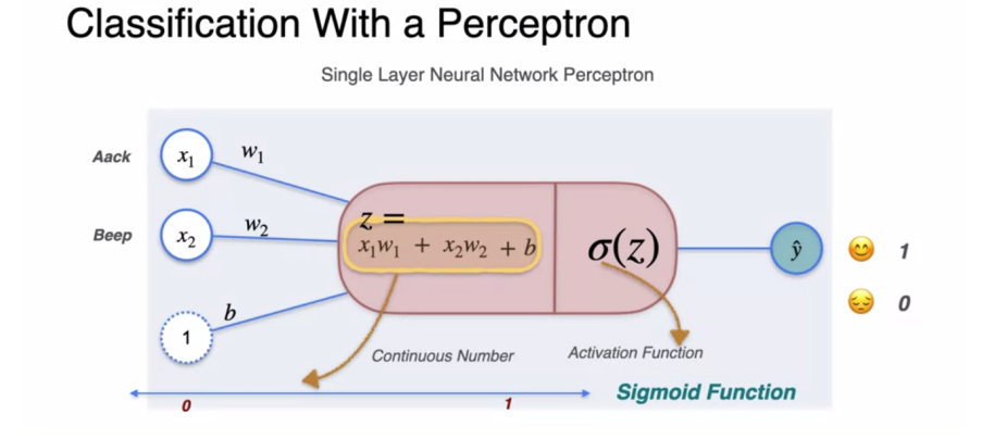
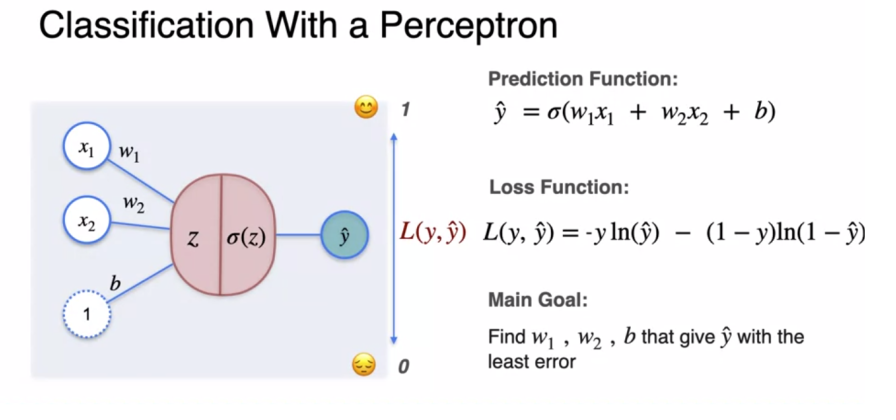
This section covers the basic building block of neural network which is perceptron (single unit), identical activation function along with using perceptron for regression, sigmoid activation along with using perceptron for classification.

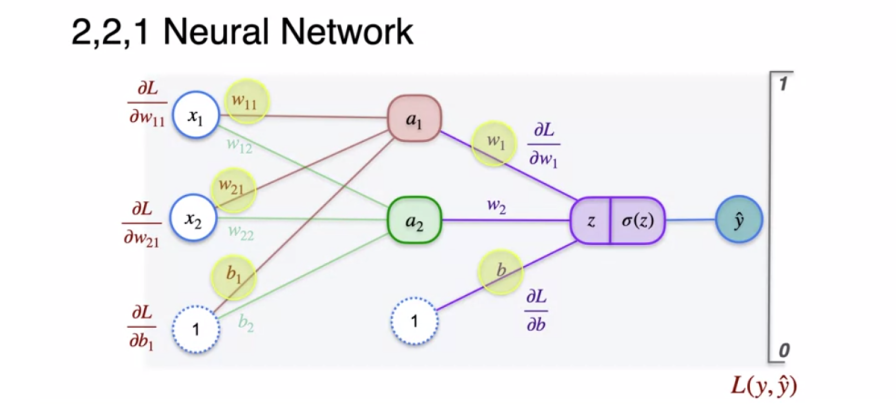
Next, how multiple perceptron along with non-linear activations help to create non-linear or complex data patterns which gives us powerful Neural networks. The beauty of neural network which mimics biological neurons comes into picture when we appreciate the beauty of activations and multiple perceptrons acting together.

#Perceptron + Classification

#Importance of Activations and its role in non-linearity

• Activation is key for artificial neural network to be actual artificial neural network
• Without non-linear activations, artifical neural networks irrespective of number of layers, will still be linear
• In calculus, is the function differentiable? is vital question to ask. Linear activation functions have constant as derivative. Below section on optimization and backpropagation show some notes on importance of functions being differntiable.
• Choosing the right activation functions for the output layer, hidden layers varies based on the dataset, context of problem for example, Multi-class classification, RNN, CNN, GANs etc

In neural networks, non-linear boundaries and planes refer to the decision surfaces created by the network to separate different classes in the data. Unlike linear models (like logistic regression) that can only create straight lines or hyperplanes for classification, neural networks with non-linear activation functions can learn more complex boundaries to better fit intricate data patterns.

#Linear vs. Non-Linear Decision Boundaries:

Linear Decision Boundaries: Imagine a simple classification task where you want to separate red and blue dots in a two-dimensional space. A linear model can only draw a straight line to achieve this separation. This line represents the decision boundary – any point above the line might be classified as red, and any point below it might be classified as blue.

Non-Linear Decision Boundaries: However, real-world data is often more complex. Consider data points that aren’t neatly separated by a straight line. Here’s where non-linear decision boundaries come into play. Neural networks with non-linear activation functions, like ReLU or sigmoid, can create more intricate boundaries. These boundaries can be curves, circles, or more complex shapes that better fit the underlying data distribution.

• Activation Functions: The key to non-linearity lies in the activation functions used in the hidden layers of a neural network. These functions introduce non-linear transformations on the data as it flows through the network. Common activation functions include:

  • ReLU (Rectified Linear Unit): Outputs the input itself if it’s positive, otherwise outputs zero. This allows the network to learn “piecewise linear” boundaries by stacking multiple ReLU layers.
  • Sigmoid: Squeezes the input value between 0 and 1, introducing a sigmoidal curve as the decision boundary.
  • Tanh (Hyperbolic Tangent): Similar to sigmoid but squashes the output between -1 and 1, creating a smoother S-shaped boundary.

There are other non-linear activation functions getting invented and already invented for a specific purposes. For example, GELU. In this post, I am not planning to write about other non-linear activations.

Multiple Layers: By stacking multiple hidden layers with non-linear activation functions, neural networks can combine these non-linear transformations to create even more complex decision boundaries. Each layer learns a slightly different non-linearity, and the combined effect allows the network to fit intricate data patterns.

#Benefits of Non-Linear Boundaries:

One of the benefits which I like to highlight for the context

Feature Extraction: As a hidden layer learns a non-linear transformation, it might be implicitly extracting higher-order features from the input data. These features can be more informative for classification compared to the raw input features.

Let me touch upon common activation functions without going into details.

• Linear Activation (f(x) = x):

  • This function simply outputs the input value.

• Sigmoid Activation (f(x) = 1 / (1 + exp(-x))):

  • Outputs a value between 0 and 1, with a gradual S-shaped curve.

• ReLU Activation (f(x) = max(0, x)):

  • Outputs the input if it’s positive, otherwise outputs zero.

• Hyperbolic Tangent (tanh) Activation (f(x) = (exp(x) - exp(-x)) / (exp(x) + exp(-x))):

  • Outputs a value between -1 and 1, with a smoother S-shaped curve compared to sigmoid.

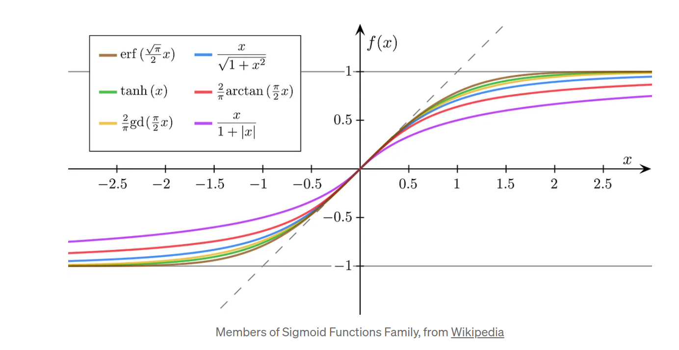
• I am not planning to go deep on derivatives of different non-linear activation functions described above. All we need to know is they are differentiable.

#Multiple Perceptrons

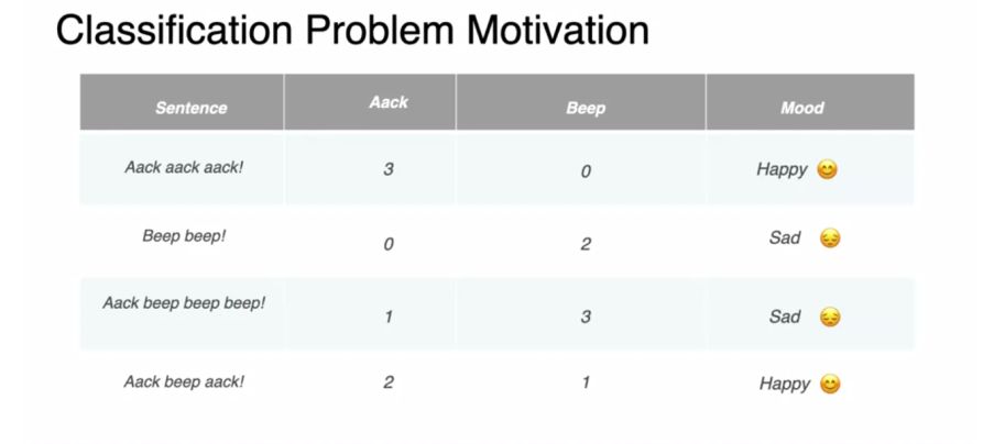
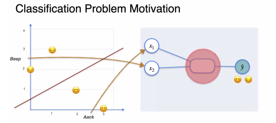
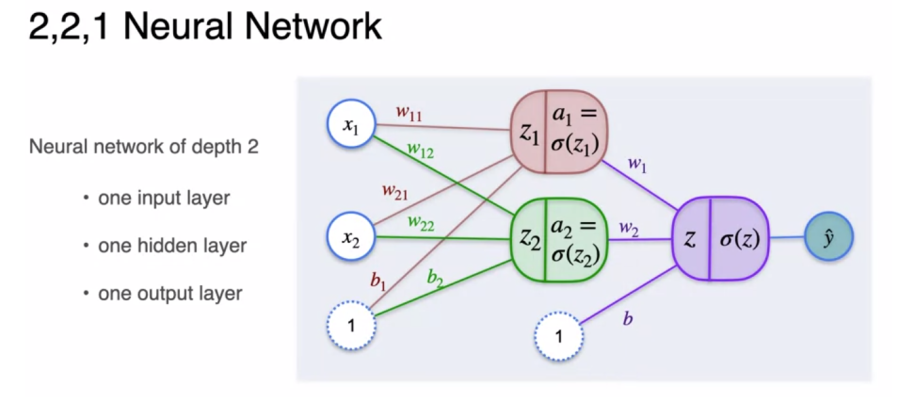
I like to view neural network as bunch of perceptrons organized in layers where the information gets selectively passed between layers. This post is not about just neural networks or any specific models but the role of calculus. In the above perceptron for classificatin, I shared the particular example to show linear boundary, a line between happy and sad sentences. In reality, we all know that language is not filled with words Beep, Aack. So the dimensionality increases multi-fold in reality and multiple perceptrons (neural network) along with appropriate activation helps in non-linear separation of happy and sad sentences in the context of above example.

#Optimizations

There are two main branches of continous optimization. In machine learning, objective functions has to differentiable as stated before. By convention, most objective functions in machine learning are intended to be minimized, that is, the best value is the minimum value. Intuitively finding the best value is like finding the valleys of the objective function, and the gradients point us uphill. The idea is to move downhill (opposite to the gradient) and hope to find the deepest point.

• Unconstrained => Gradient Descent => Stepsize, Momentum, Stochastic Gradient Descent.
• Constrained => Lagrange Multipliers

Gradient descent is a first-order optimization algorithm. To find a local minimum of a function using gradient descent, one takes steps proportional to the negative of the gradient of the function at the current point. Recall from Section 5.1 that the gradient points in the direction of the steepest ascent. Another useful intuition is to consider the set of lines where the function is at a certain value (f (x) = c for some value c ∈ R), which are known as the contour lines. The gradient points in a direction that is orthogonal to the contour lines of the function we wish to optimize.

Step-Size

• If the step-size is too small, gradient descent can be slow. If the step-size is chosen too large, gradient descent can overshoot, fail to converge, or even diverge.

If the step-size is too small, gradient descent can be slow. If the step-size is chosen too large, gradient descent can overshoot, fail to converge, or even diverge.

• If the step-size is too small, gradient descent can be slow. If the step-size is chosen too large, gradient descent can overshoot, fail to converge, or even diverge
• When the function value decreases the step could have been larger. Try to increase the step-size.

Momentum

• The momentum-based method remembers the update ∆xi at each iteration i and determines the next update as a linear combination of the current and previous gradients.

Stochastic Gradient Descent

• Stochastic gradient descent (often shortened as SGD) is a stochastic approximation of the gradient descent method for minimizing an objective function that is written as a sum of differentiable functions. The word stochastic here refers to the fact that we acknowledge that we do not know the gradient precisely, but instead only know a noisy approximation to it.
• Standard gradient descent, as introduced previously, is a “batch” optimization method, i.e., optimization is performed using the full training set.
• In contrast to batch gradient descent, which uses all Ln for n = 1, … , N , we randomly choose a subset of Ln for mini-batch gradient descent. In the extreme case, we randomly select only a single Ln to estimate the gradient.

In the realm of optimization problems, Lagrange multipliers come into play when we want to optimize a function (often maximizing something like profit or minimizing something like cost) while adhering to certain limitations or rules. These limitations are formulated as constraints. There are two main types of constraints we can encounter:

Equality Constraints: These constraints specify an exact relationship between variables. They are often written in the form of equations like f(x, y, z) = 0, where f represents a function and x, y, and z are variables. Inequality Constraints: These constraints define boundaries or limitations on the values a variable can take. They are typically expressed as inequalities like g(x, y, z) ≤ h(x, y, z) or g(x, y, z) ≥ h(x, y, z), where g and h represent functions and x, y, and z are variables. Lagrange Multipliers and Inequality Constraints:

While Lagrange multipliers are generally used to solve problems with equality constraints, there’s a technique to incorporate them into problems with inequality constraints as well. This approach involves introducing a new concept: slack variables.

Slack Variables: These are artificial variables introduced to convert an inequality constraint into an equality constraint. They are non-negative (always greater than or equal to zero) and essentially take up the “slack” in the inequality, allowing us to apply the Lagrange multiplier method.

In the context of optimization problems with Lagrange multipliers, duality is a fascinating concept that reveals a deeper connection between the original problem (primal problem) and a newly formed problem (dual problem). Here’s a breakdown of the key aspects:

The Primal Problem and Constraints:

Imagine you’re running a factory and want to minimize your production costs (objective function). However, you also have limitations, such as:

Production capacity: You can’t produce more than a certain amount (represented by an inequality constraint). Labor regulations: You need to adhere to minimum working hours for your employees (another inequality constraint). These limitations are formulated as constraints in the optimization problem you’re trying to solve.

Introducing Lagrange Multipliers:

Lagrange multipliers (λ) are introduced to handle these constraints. They act as “weights” on the constraints, penalizing solutions that violate them. The goal becomes to minimize the original objective function while also considering the penalty imposed by the Lagrange multipliers for violating the constraints.

The Lagrangian Function:

The Lagrangian function (L) combines the original objective function (f) with the constraints multiplied by their respective Lagrange multipliers:

L(x, λ) = f(x) + Σ λᵢ * gᵢ(x) (where x represents the decision variables, λᵢ are Lagrange multipliers, and gᵢ are the constraint functions)

Solving the Primal Problem:

We find the values of the decision variables (x) and Lagrange multipliers (λ) that minimize the Lagrangian function. This solution satisfies the constraints and provides the optimal solution for the original minimization problem (primal problem).

The Dual Problem:

Now comes the duality aspect. Based on the primal problem and its Lagrangian function, we can define a new optimization problem called the dual problem. The dual problem aims to:

Maximize a function of the Lagrange multipliers (λ): This function, often denoted by g(λ), is constructed based on the primal problem’s constraints and objective function. Subject to certain constraints on the Lagrange multipliers (λ): These constraints might involve ensuring the Lagrange multipliers are non-negative (if they correspond to inequality constraints in the primal problem).

#Gradient Descent + Perceptrons

Now we have seen constrained optimization and unconstrained optimization. Next it is important to refer to different loss functions, role of unconstrained optimization (Gradient Descent) before we take a deeper look at famous automatic differentiation.

Some refer to cost as loss of entire training set and loss as individual training sample. Some interchange loss and cost.

My goal is not to replicate or write in detail about loss functions. There are lots of great posts about loss functions and summary of activation functions. Please find few in reference below. With practise, it is easy to remember different loss functions. For example, how and when to use binary cross entropy loss for binary classification, using log softmax + negative log likelihood or Cross entropy loss for multi class classification.

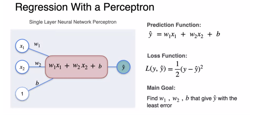
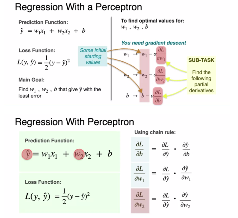
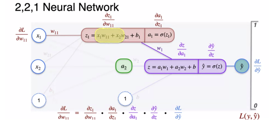
Following gives an idea to calculate partial derivates of loss functions with respect to weights and biases.

Gradient Descent

Quick Recap - So far we have seen importance of activation functions, non-linearity which enables multiple dimension of features. At this point we know there are weights and biases, which takes inputs and calculate sum of their products, then activation functions activates what is needed and pass to next layer (in context of multiple perceptron layers). Above is forward pass and we calculate loss at the end. We saw how to calculate gradients of loss with respect to weights and biases.

#Backpropagation

Backward pass helps us to see how loss varies with updated weights and biases. Here comes the role of unconstrained optimization which uses gradients of loss with respect to weights and biases to update the weights and biases. You will see everywhere the famous ball rolling down the hill or someone trying to go down the hill to final optimistically global minium or lowest point of the hill.

• We have seen above how gradient descent updates the weight and biases. In this section, my goal is to highlights the fact that if you look at gradient chain backward or traverse from root to leaves where leaves are inputs, root is final output where we calculate loss.

• Let us take a simple network like below

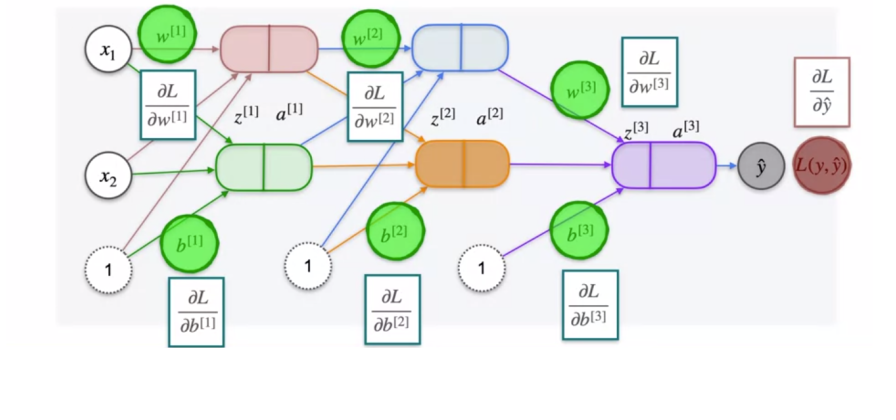
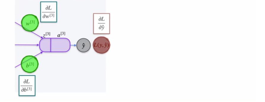
• Pay attention to how partial derivative of how loss varies with respect to W3 can be calculated with partial derivatives calculated in backward direction a —> z —> w3

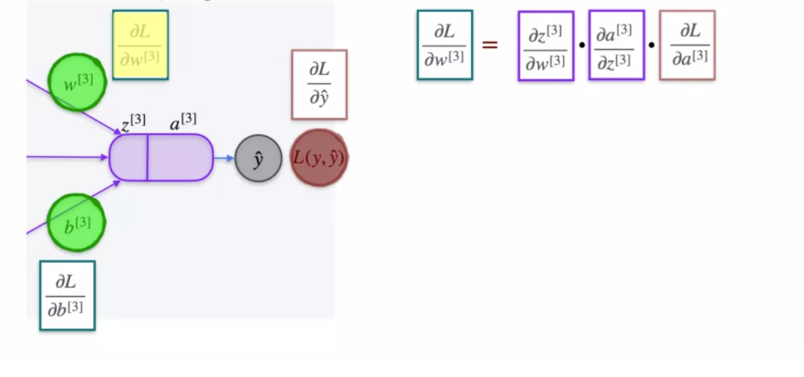
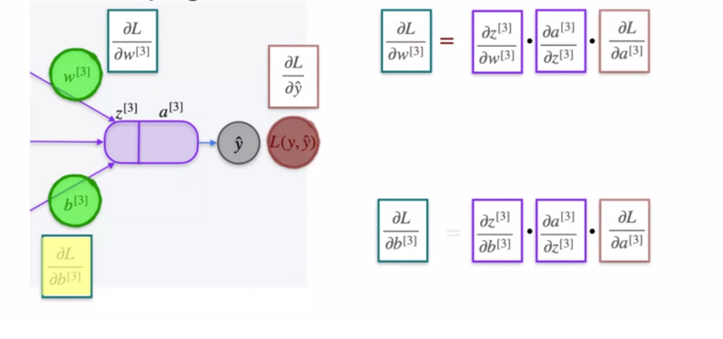
• Just showing a longer chain backwards L —> a3 —> z3 —> a2 -> z2 —> a1 —> z1 —> w1

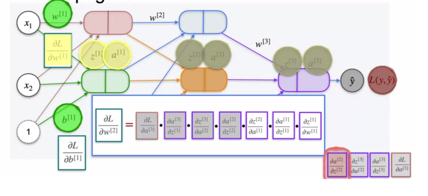
Remember regular batch gradient descent varies from stochastic (single randomnly selected sample) varies from mini-batch gradient descent (randomnly selected subset of training examples at each iteration)

If you ask your favorite code generating model, the following code gets generated which is self explanatory for linear regression, squared loss (cost), calculating partial derivates respect to weight and bias. Then gradient descent (update weight and bias to check how loss varies)

• I have asked Google Gemini to generate gradient function for linear regression and here is the generated code

import numpy as np

def gradient_descent(X, y, learning_rate, num_iterations):
  """
  Performs gradient descent to find the optimal weights for linear regression.

  Args:
      X: A numpy array of shape (m, 1) representing the features.
      y: A numpy array of shape (m,) representing the target values.
      learning_rate: The learning rate for gradient descent.
      num_iterations: The number of iterations to perform gradient descent.

  Returns:
      A tuple containing the learned weights (w) and the bias (b).
  """

  m = len(X)  # Number of training examples

  # Initialize weights with zeros
  w = np.zeros(shape=(1,))
  b = 0

  # Perform gradient descent for the specified number of iterations
  for iteration in range(num_iterations):
    # Calculate predictions
    predicted_y = w * X + b

    # Calculate the error
    error = predicted_y - y

    # Calculate the gradients
    dw = (1 / m) * np.sum(X * error)
    db = (1 / m) * np.sum(error)

    # Update weights and bias
    w -= learning_rate * dw
    b -= learning_rate * db

  return w, b

# Example usage
X = np.array([[1], [2], [3], [4]])
y = np.array([2, 4, 5, 6])

learning_rate = 0.01
num_iterations = 1000

w, b = gradient_descent(X, y, learning_rate, num_iterations)

print(f"Learned weights: {w[0]}")
print(f"Learned bias: {b}")

#Automatic Differentiation

Let me first share what is automatic differentiation and why famous deep learning frameworks call them autodiff, autograd etc.

• The gist is calculating gradients of function should be as easy or in other words computationaly same level of complexity, as calculating the function value itself. We can also say, rules for transforming the code for function into code for gradient should be equal complexity.

Formal Definition Wikipedia - Automatic differentiation exploits the fact that every computer calculation, no matter how complicated, executes a sequence of elementary arithmetic operations (addition, subtraction, multiplication, division, etc.) and elementary functions (exp, log, sin, cos, etc.). By applying the chain rule repeatedly to these operations, partial derivatives of arbitrary order can be computed automatically, accurately to working precision, and using at most a small constant factor of more arithmetic operations than the original program.

For folks who are interested to read more about constrained perspective (equality constraint) of autodiff Autodiff by the method of Lagrange Multipliers

It turns out that backpropagation is a special case of a general technique in numerical analysis called automatic differentiation. We can think of automatic differentation as a set of techniques to numerically (in contrast to symbolically) evaluate the exact (up to machine precision) gradient of a function by working with intermediate variables and applying the chain rule. Automatic differentiation applies a series of elementary arithmetic operations, e.g., addition and multiplication and elementary functions, e.g., sin, cos, exp, log. By applying the chain rule to these operations, the gradient of quite complicated functions can be computed automatically.

• Automatic differentiation can be both forward and backward. However, in the context of neural networks, where the input dimensionality is often much higher than the dimensionality of the labels, the reverse mode is computationally significantly cheaper than the forward mode.

I like the following explanation from my favorite math for maching learning book (check reference)

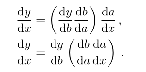
First equation would be the reverse mode because gradients are propagated backward through the graph, i.e., reverse to the data flow. Second equation above would be the forward mode, where the gradients flow with the data from left to right through the graph.

By thinking of each of the derivatives above as a variable, we can observe that the computation required for calculating the derivative is of similar complexity as the computation of the function itself

#Conclusion

Lot of notes. Finally its time to wrap up my understanding of calculus in the context of machine learning. Following keywords are the gist of this entire post

• Jacobians
• Jacboain vector products
• Determinant of Jacobian matrix
• First-order derivatives
• Different optimization techniques.
• Perceptron (single unit)
• Multiple perceptron
• Importance of non-linearity and role of activation functions
• Different loss functions.
• Forward propagation, Backward propagation
• Automatic Differentiation

#Resources

• Watch the first two videos to motivate yourself about activations involved in artifical neural networks, my favorite 3B3B
• My another favorite author Cohal’s
• Why Momentum works
• Pytorch Autograd
• Pytorch Autograd Mechanics
• JAX Autodiff
• JAX Autograd
• Tensorflow’s Autodiff
• Mathematics For Maching Learning - My favorite book
• Loss Functions Cheat Sheet
• Cross Entrophy
• Loss Functions
• Killer Combo