Essence of Linear Algebra using 100+ years old PCA (Principal Component Analysis)

This post is part of yet-another series where I write about classical algorithms or topics in my own words, understandings, captured notes from great sources.

Linear algebra is one of the core mathematical concepts needed to effectively understand machine learning, deep learning algorithms.

After completing wonderful courses on necessary math for machine and deep learning from following great sources

Mathematics for Machine learning specialization - Imperial College London
Mathematics for Machine learning and Data Science Specialization - Coursera by my favorite Lois Serrano
My favorite 3 blue 1 Brown
Best book Mathematic For Machine Learning

I was thinking about one topic which can be a good epitome of Linear Algebra concepts. Nothing better than 100+ years algorithm PCA which is still widely used.

This post covers topics from all the above sources and I will share my personal hand written notes along with some insights on PCA. I strongly believe this one algorithm covers most of the important topics of Linear Algebra necessary for a Data scientist or Deep learning engineer.

We will discuss principal component analysis (PCA), an algorithm for linear dimensionality reduction. PCA, proposed by Pearson (1901) and Hotelling (1933), has been around for more than 100 years and is still one of the most commonly used techniques for data compression and data visualization.

I like the approach taken by MML book to explain PCA which follows different perspectives to explain the math behind PCA. My favorite versions are latent view perspective, variance perspective and projection perspective.

Unveiling Hidden Patterns: Principal Component Analysis (PCA)

Principal Component Analysis (PCA) is a cornerstone technique in data science, allowing us to explore and understand high-dimensional datasets. At its core, PCA aims to identify a smaller set of features, called principal components (PCs), that capture the most significant variations within the data. This allows us to represent the data in a lower-dimensional space while retaining most of the information.

The Power of Variance: Capturing the “Spread” of the Data Imagine a dataset representing customer purchases at a grocery store. Each data point could describe a customer, with features like the amount spent on vegetables, fruits, dairy products, and so on. PCA helps us identify the directions (principal components) in this high-dimensional space that exhibit the most significant spread or variance in customer spending habits.

Here’s a breakdown of the key concepts:

Data Matrix (X): This matrix holds our data, where each row represents a data point (customer) and each column represents a feature (spending on a specific category). Centered Data: Often, PCA involves centering the data by subtracting the mean vector from each data point. This ensures our analysis focuses on the variations around the mean, not the absolute values. Unveiling the Structure: Eigenvalue Decomposition and Covariance Matrix PCA leverages the power of linear algebra to achieve dimensionality reduction. Here’s the mathematical connection:

Covariance Matrix (Σ): This matrix captures the linear relationships between features in the data. It tells us how much each feature co-varies with the others.

Eigenvalue Decomposition: Decomposing the covariance matrix reveals its eigenvalues (λᵢ) and eigenvectors (vᵢ).

Eigenvalues are non-negative real numbers representing the variance along the direction of the corresponding eigenvector. The larger the eigenvalue, the greater the variance in that direction. Eigenvectors are orthogonal vectors (meaning perpendicular in this high-dimensional space) that define directions within the data. Key Point: Eigenvalues tell us how “spread out” the data is along a specific direction defined by the eigenvector.

Unveiling the Structure (Alternative Approach): Singular Value Decomposition (SVD) While PCA can be formulated using eigenvalue decomposition of the covariance matrix (Σ), SVD offers a more general and computationally efficient approach:

SVD of the Data Matrix: SVD can be performed directly on the centered data matrix (X) to reveal:

X = UΣV^T where:

U (n x m) and V^T (m x m) are orthogonal matrices. Σ (n x m) is a diagonal matrix containing the singular values (σ_i) of X on its diagonal, arranged in decreasing order (σ_1 ≥ σ_2 ≥ … ≥ σ_min(m,n)). Singular Values and Eigenvalues: Interestingly, the squared singular values (σ_i²) are directly related to the eigenvalues (λᵢ) of the covariance matrix (Σ) in the following way:

λᵢ ≈ σ_i² (for centered data)

Why Use SVD for PCA?

SVD is often more efficient for calculating principal components, especially for large datasets. Singular values themselves directly represent the magnitude of variance captured by each component (no need for squaring). Selecting the Most Informative Directions: Choosing Principal Components Ordering the Components: We order the eigenvalues/singular values in descending order. This ensures the first few components capture the most significant variance in the data.

Choosing the Number of Components (k): We select the top k principal components (eigenvectors/right singular vectors corresponding to the largest eigenvalues/singular values). The choice of k depends on the desired level of information retention and dimensionality reduction.

Projecting the Data: Capturing the Essence in a Lower-Dimensional Space Projecting onto the Principal Components: Once we have chosen the k principal components, we project the data (centered or original) onto the subspace spanned by these k components. This projection gives us the principal component scores (Z), which represent the data in the lower-dimensional space defined by the principal components. Mathematically:

Z = X V_k (for centered data) Z = (X - μ) V_k (for original data) where V_k is the matrix containing the first k columns of V (right singular vectors) from the SVD.

Beyond Euclidean Distance: Kernel PCA for Non-Linear Relationships

PCA works well when the data exhibits a linear relationship in the high-dimensional space. However, real-world data often has non-linear relationships. Kernel PCA addresses this limitation by:

Mapping the data to a higher-dimensional space: It utilizes a kernel function to transform the data into a feature space where the relationships become more linear. Applying PCA in the higher-dimensional space: PCA is then performed in this transformed space to identify the principal components. Projecting back to the original space: Finally, the data points are projected back to the original space. Kernel PCA allows us to leverage the power of PCA even for data with non-linear structures.

Probabilistic PCA (PPCA): A Latent Variable Approach to Dimensionality Reduction

While Principal Component Analysis (PCA) offers a powerful technique for dimensionality reduction, it lacks a probabilistic framework. This is where Probabilistic PCA (PPCA) comes in. PPCA leverages the concept of latent variables to model the data and provide a probabilistic interpretation of the principal components.

Latent Variables: The Underlying Structure

Imagine you have a dataset representing customer purchases at a store. The observed data might include the total amount spent by each customer. However, there could be underlying factors influencing these purchases, such as:

Customer Preferences: A preference for organic products might lead to higher spending on certain categories. Seasonal Trends: Spending patterns might shift based on the season (e.g., more on fruits in summer). PPCA introduces latent variables to capture these underlying factors that influence the observed data. These latent variables are not directly observed but are inferred from the data.

The Generative Model of PPCA:

PPCA assumes the following generative process for the data:

Latent Variables: A low-dimensional vector (z) of latent variables represents the underlying factors influencing the data. Linear Transformation: The latent variables are linearly transformed by a weight matrix (W) to project them into the higher-dimensional space of observed data. Gaussian Noise: Independent Gaussian noise (ε) is added to this projection to account for measurement errors and other unexplained variations. Observed Data: The final observed data point (x) is the sum of the transformed latent variables and the noise. Mathematically, we can represent this as:

x = Wz + ε where:

x: Observed data vector (high dimensional) z: Latent variable vector (low dimensional) W: Weight matrix ε: Gaussian noise vector Benefits of the Latent Variable Approach:

Probabilistic Interpretation: PPCA allows us to estimate the probability distribution of the observed data given the latent variables. This enables tasks like anomaly detection and data imputation. Missing Data Handling: PPCA can handle missing values in the observed data by estimating the underlying latent variables.

PPCA vs. PCA: Key Differences

PCA: Focuses on maximizing variance in the data for dimensionality reduction. It doesn’t explicitly model the underlying factors influencing the data. PPCA: Introduces latent variables to capture the underlying structure and provides a probabilistic interpretation of the principal components. In essence:

PPCA builds upon PCA by introducing latent variables to model the underlying factors influencing the observed data. This probabilistic framework allows for tasks like anomaly detection, data imputation, and provides a deeper understanding of the relationships within the data.

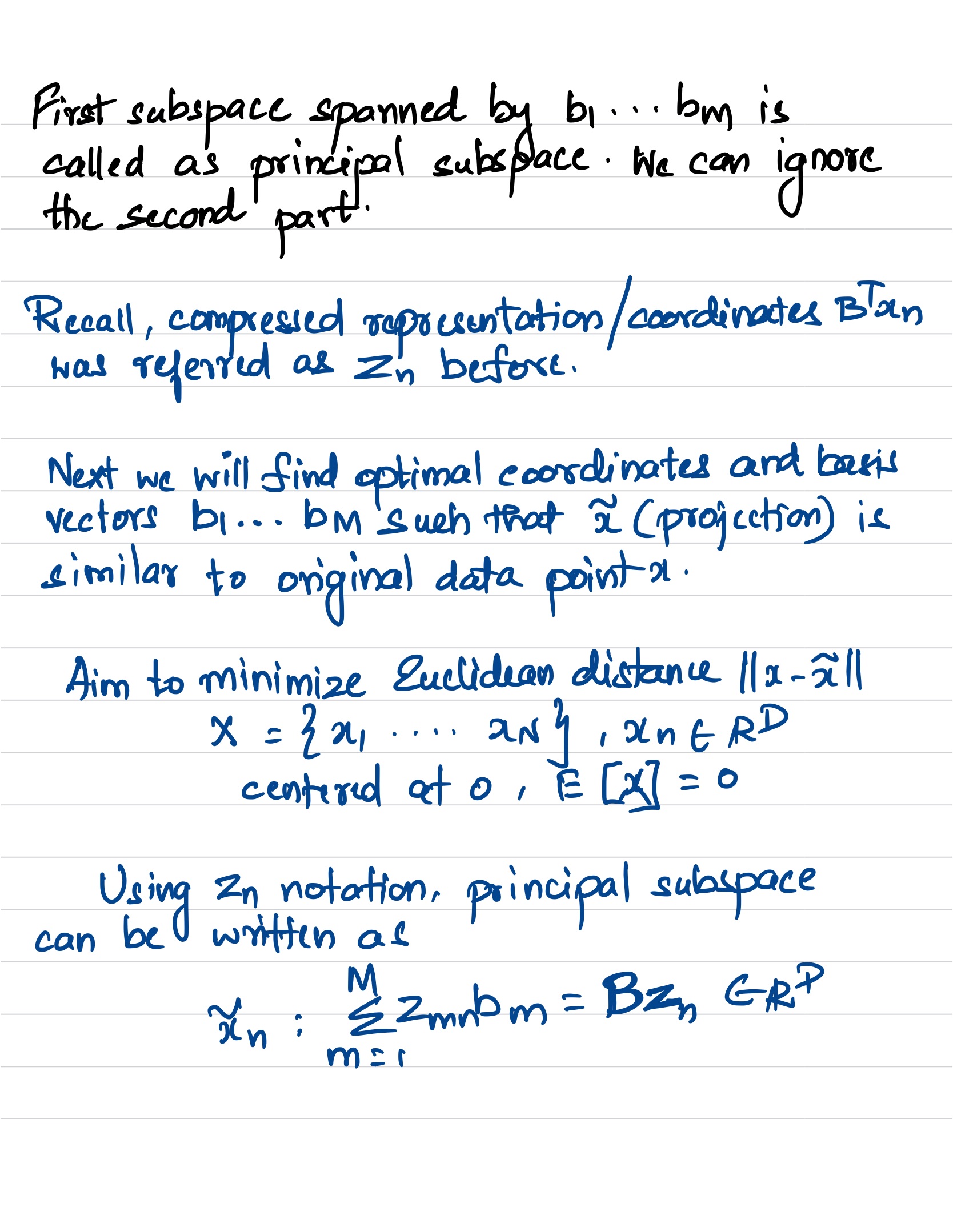
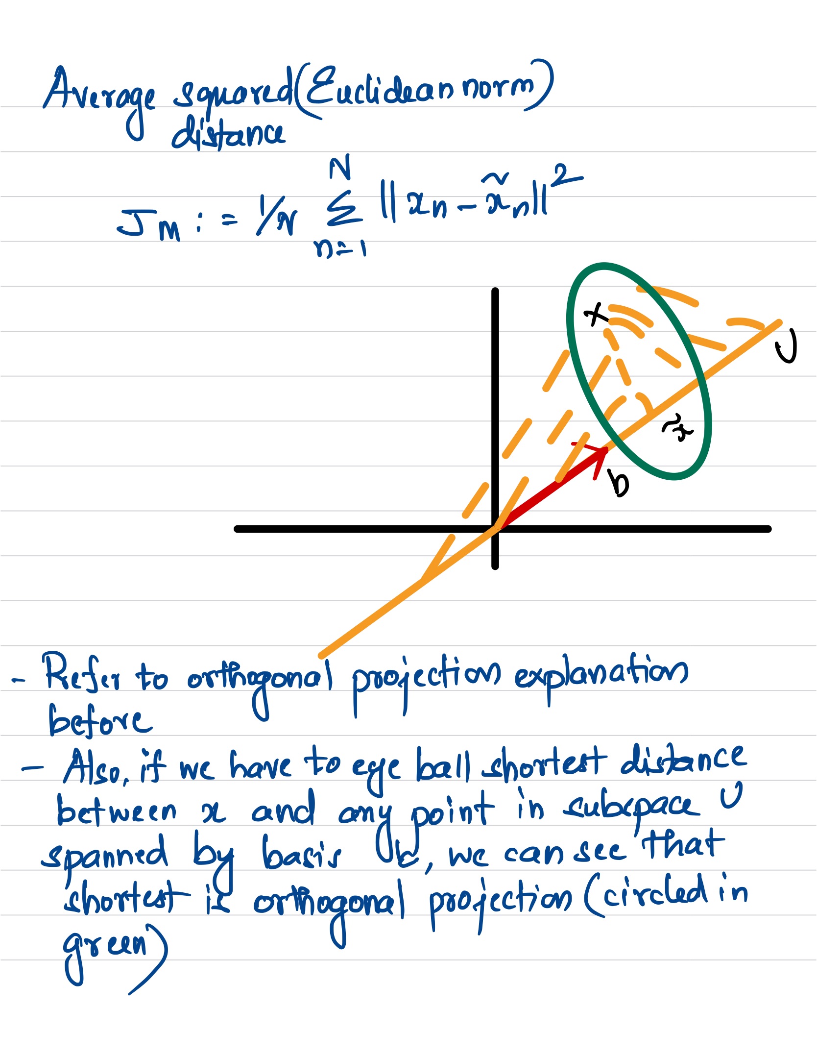
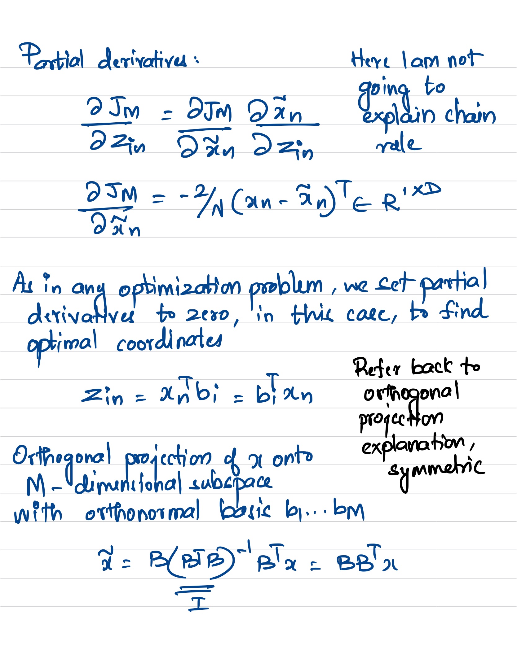
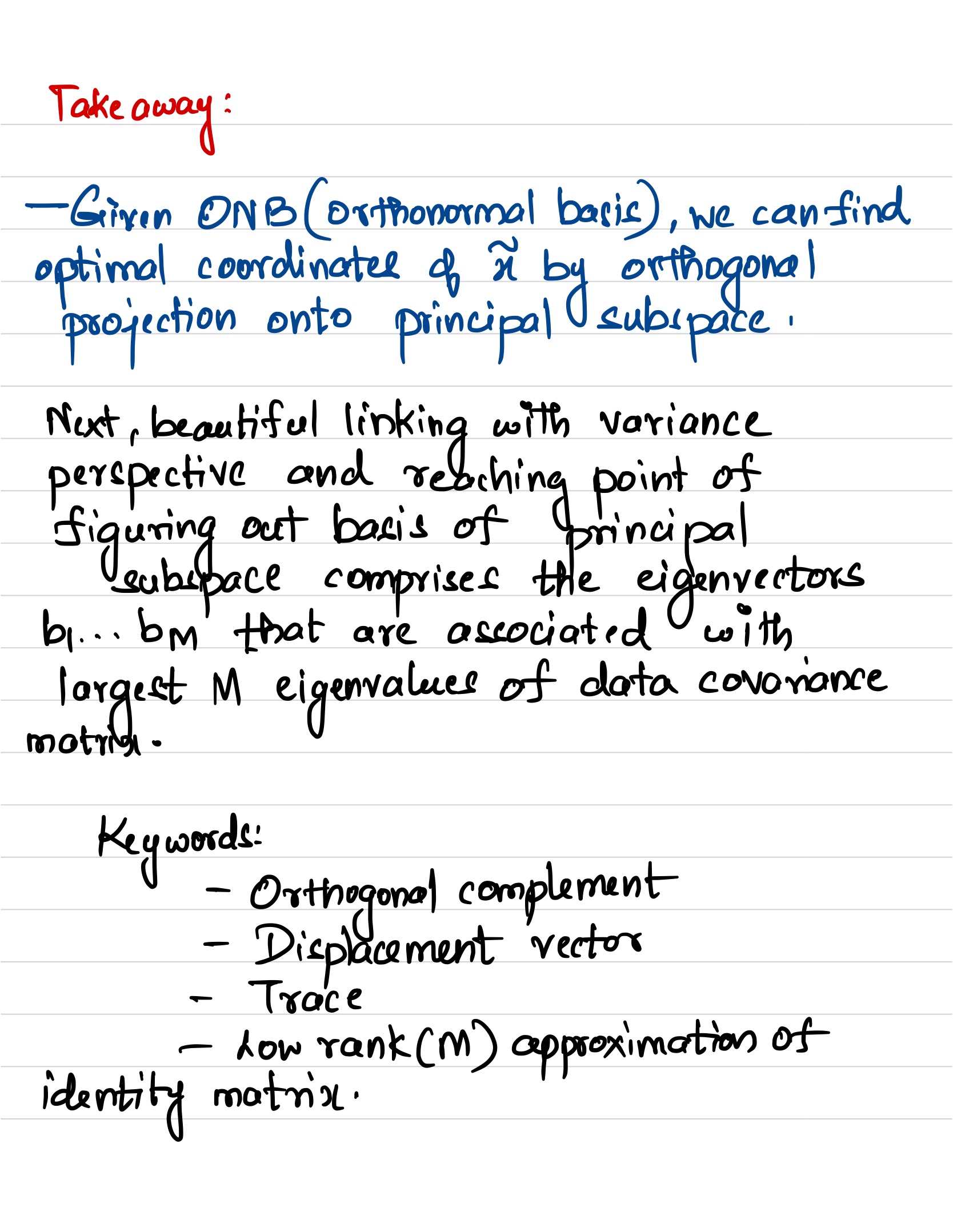
Now let us talk in depth with projection perspective and reducing reconstuction error in mind.

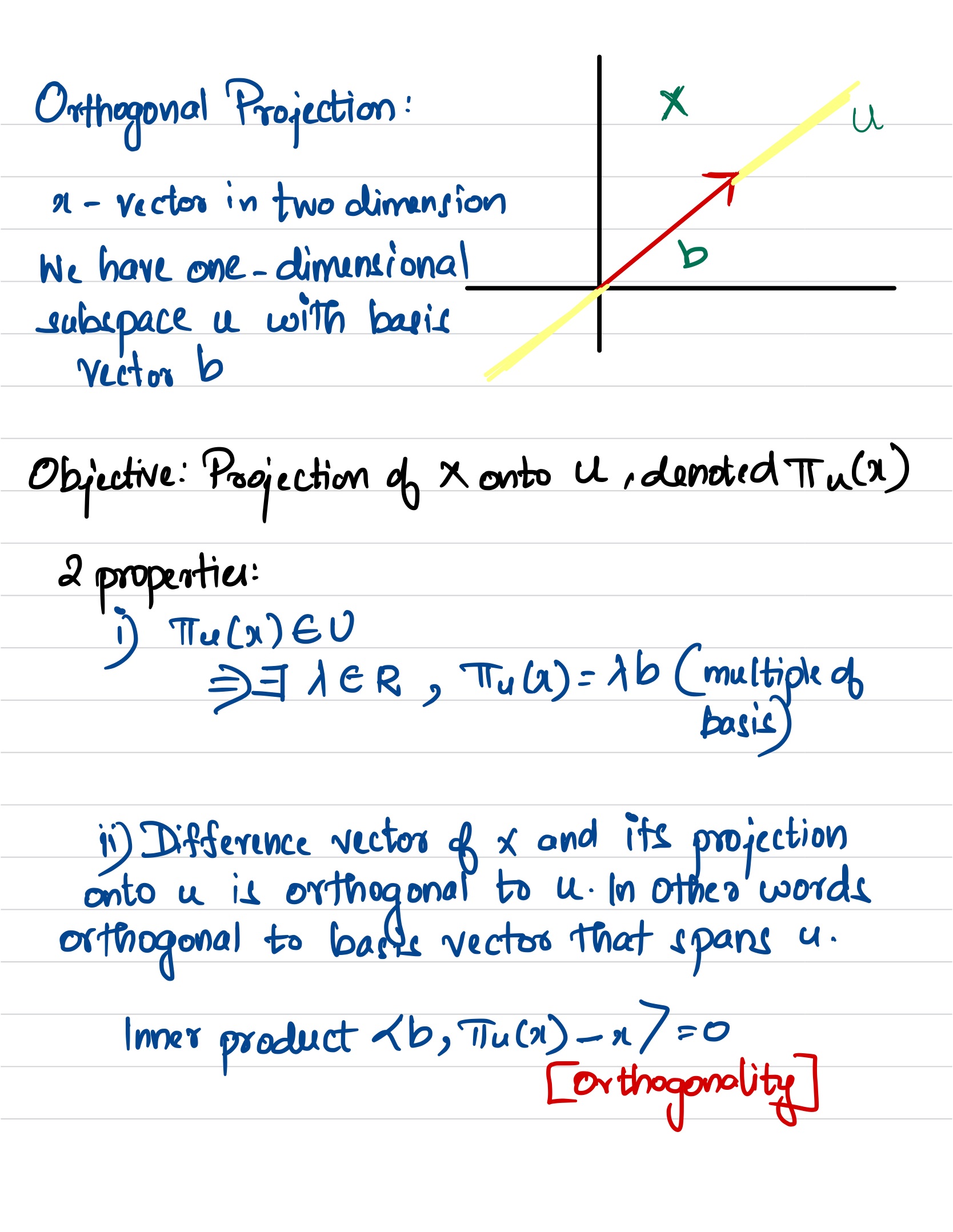
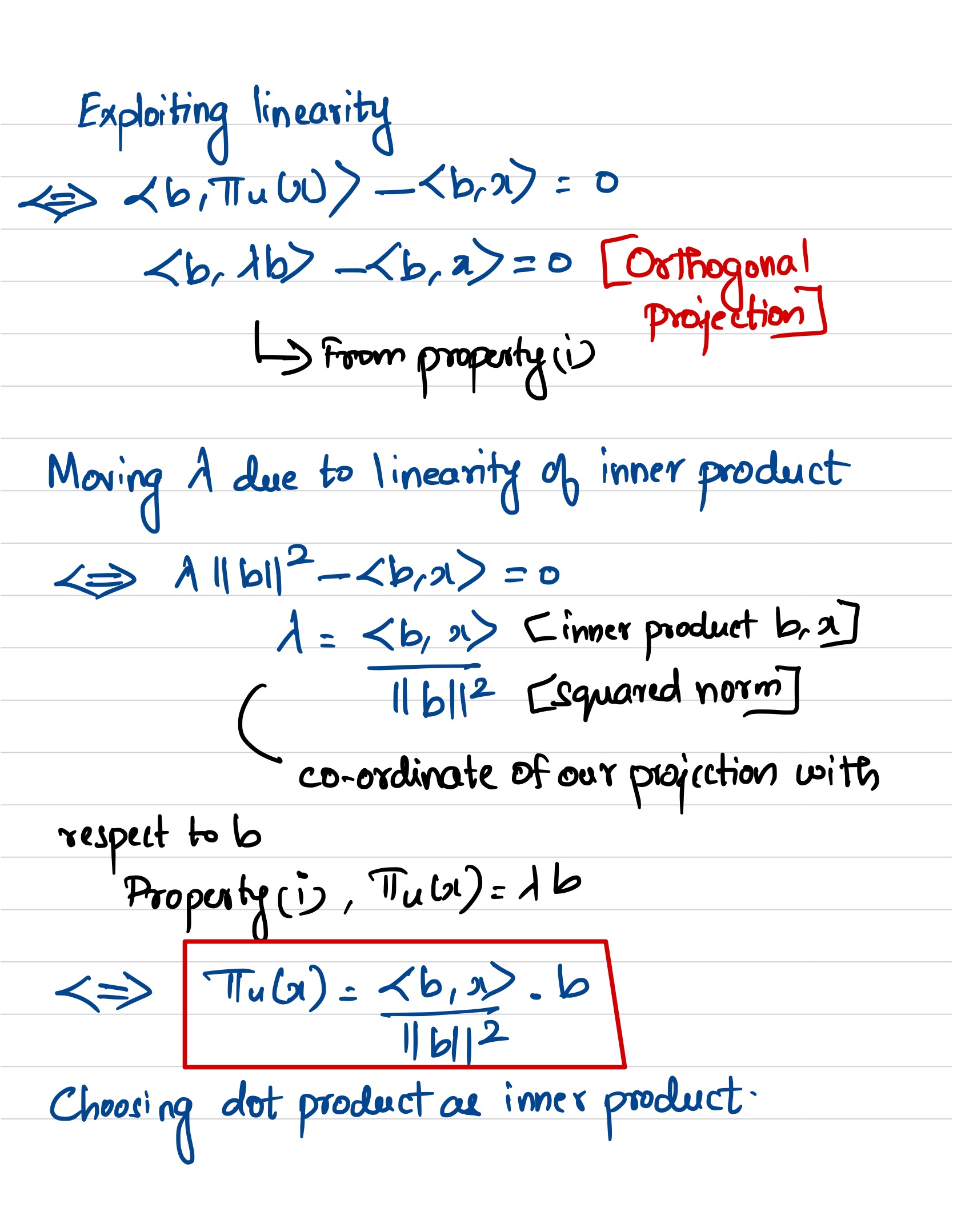
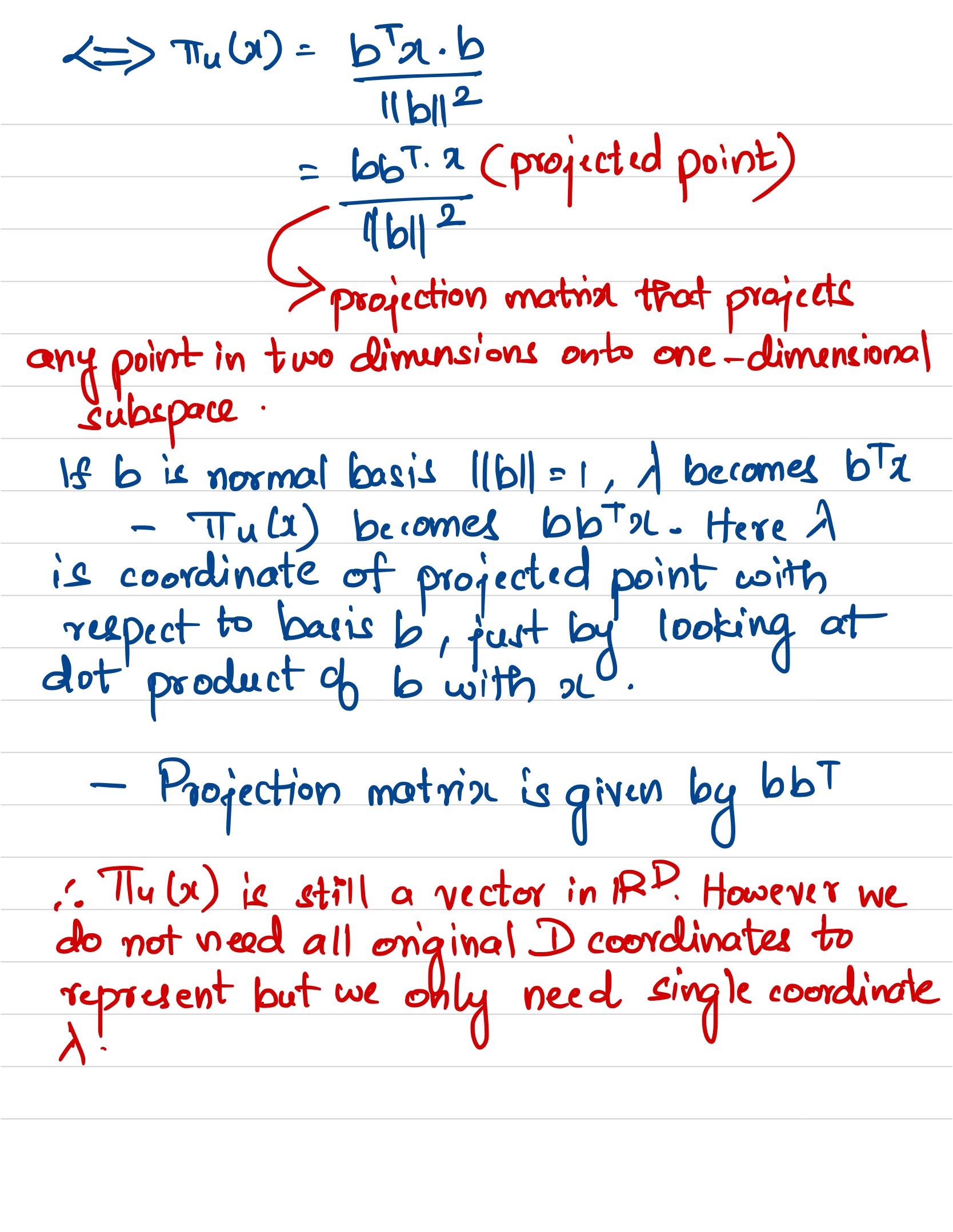
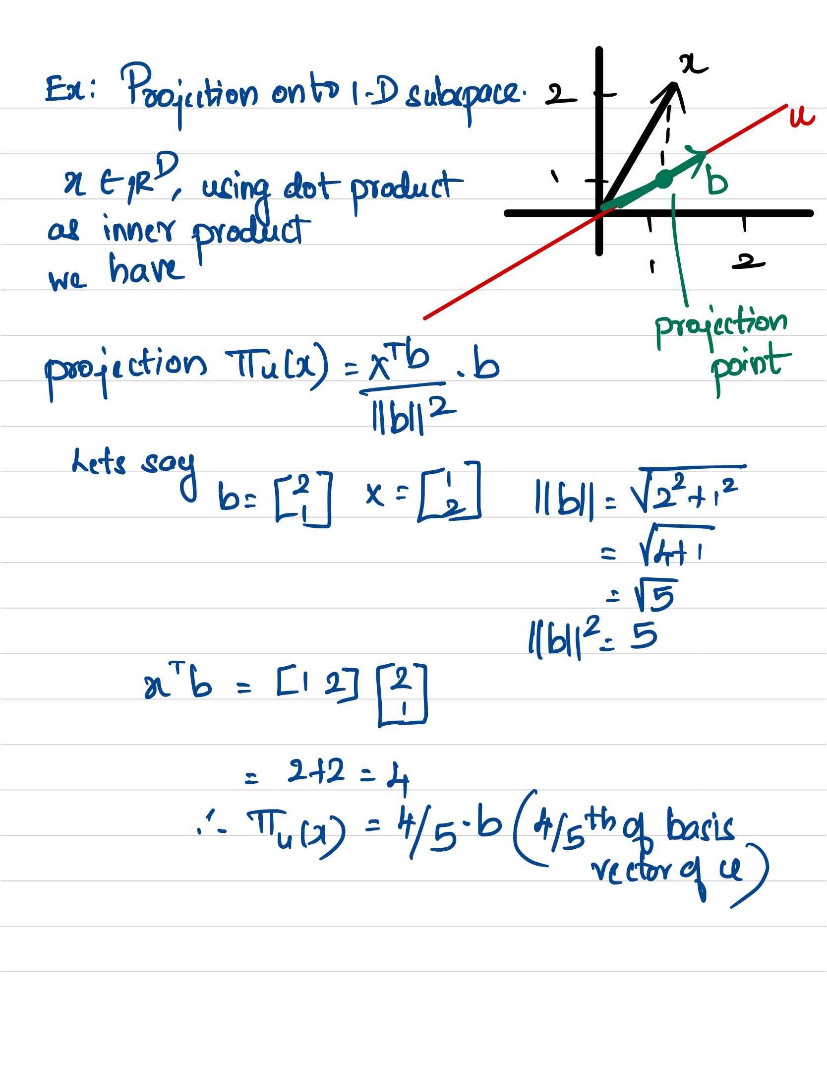
I like to first talk about Orthogonal projections with examples before I focus on projection perspective in the rest of the blog post. In later posts, I may write about latent view perspective espcially if time permits.

Orthogonal Projection 1D

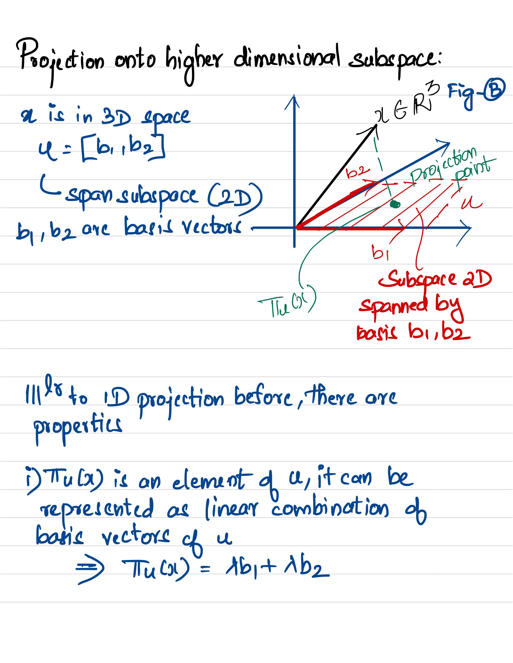
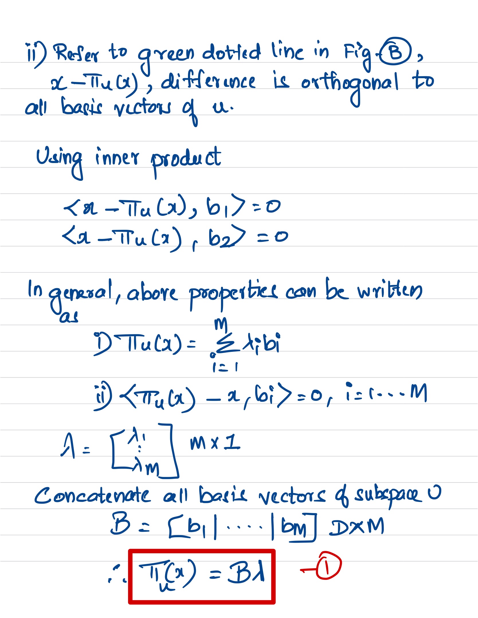
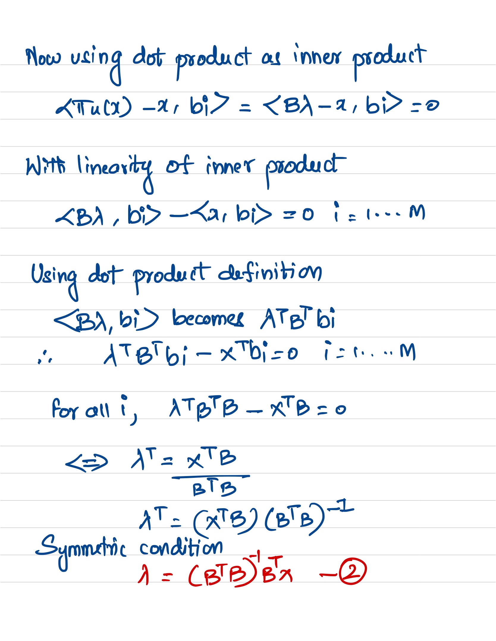
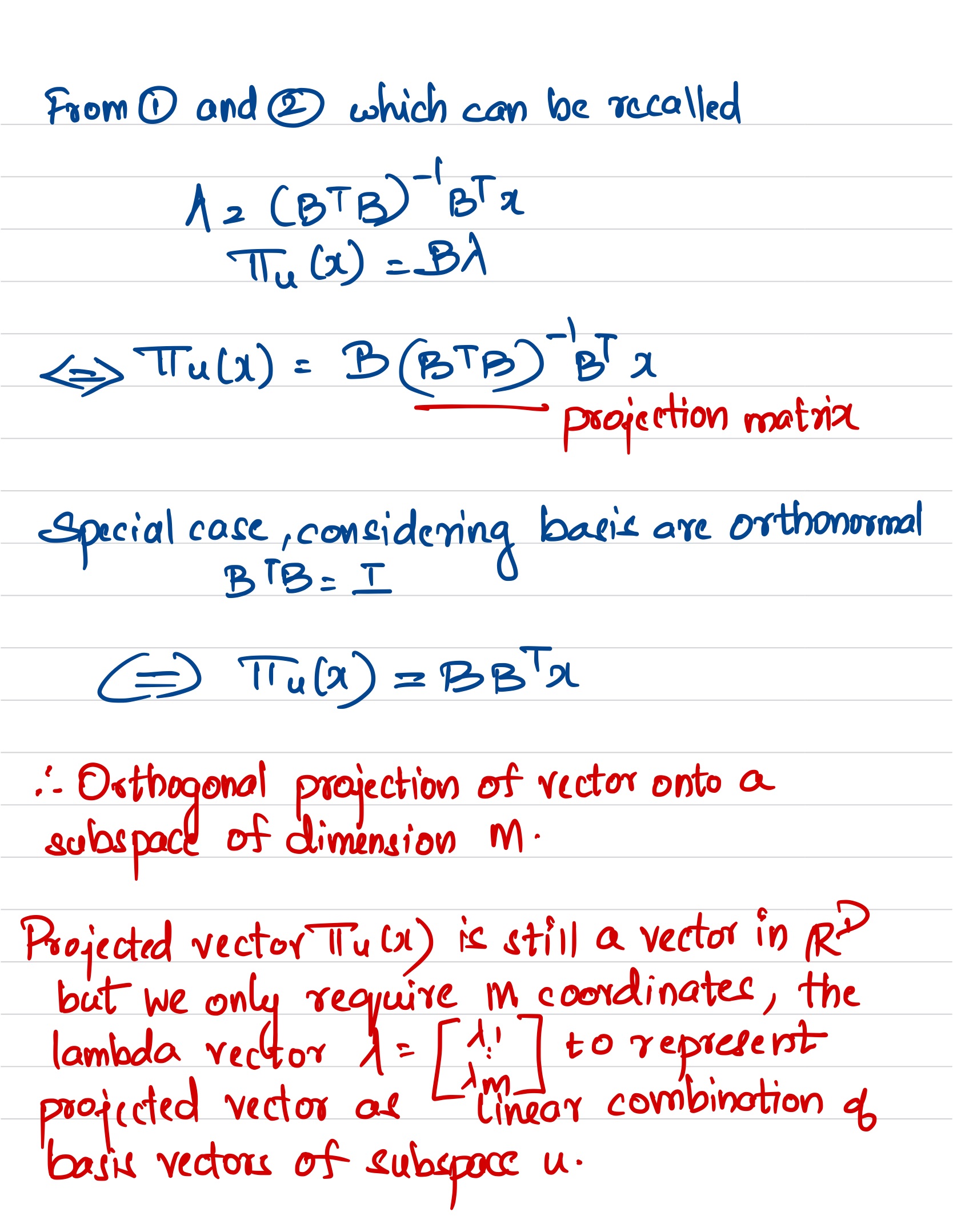
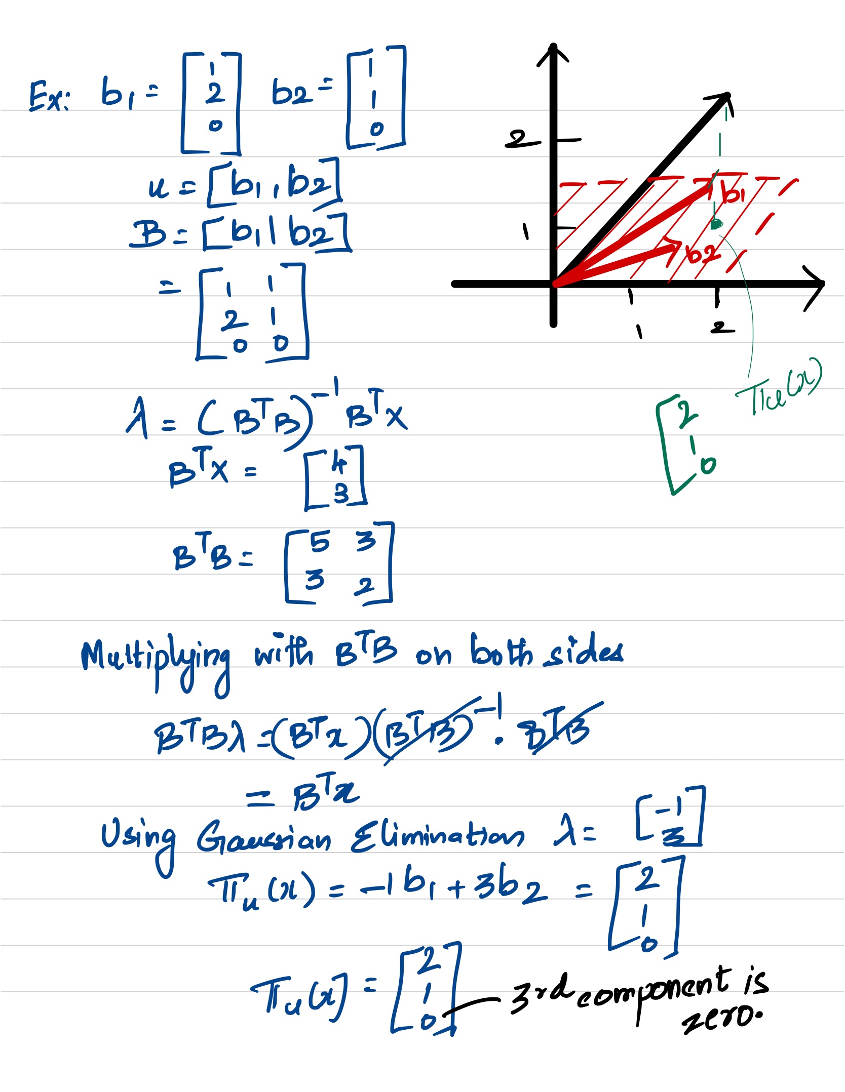
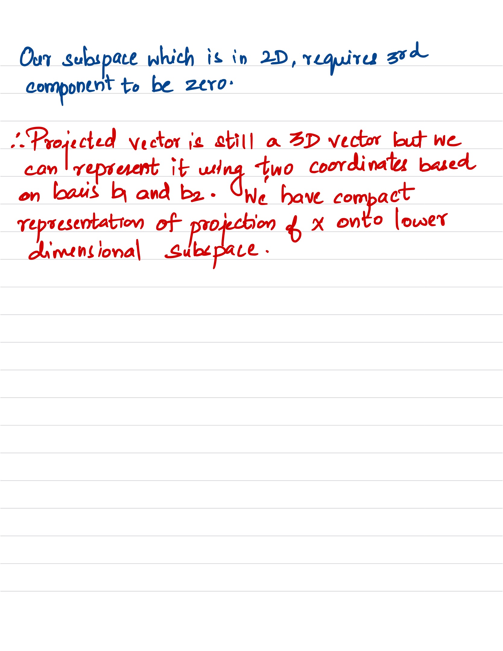
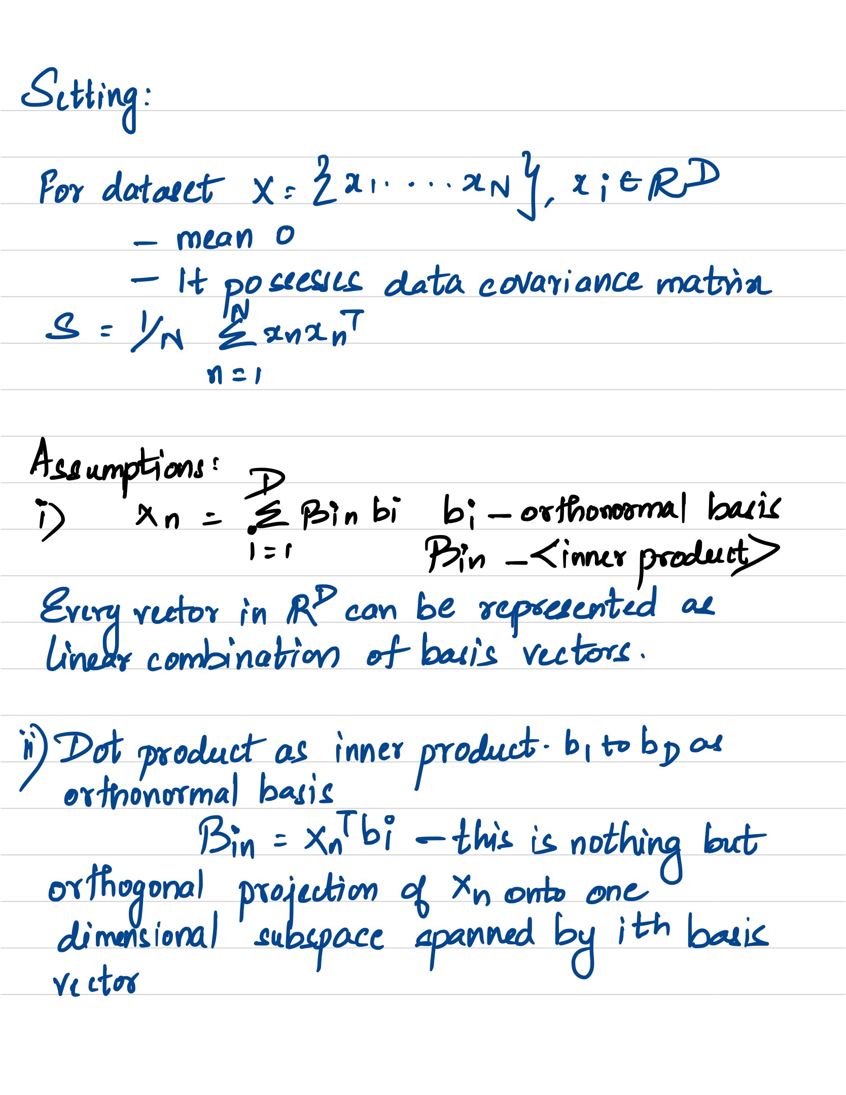
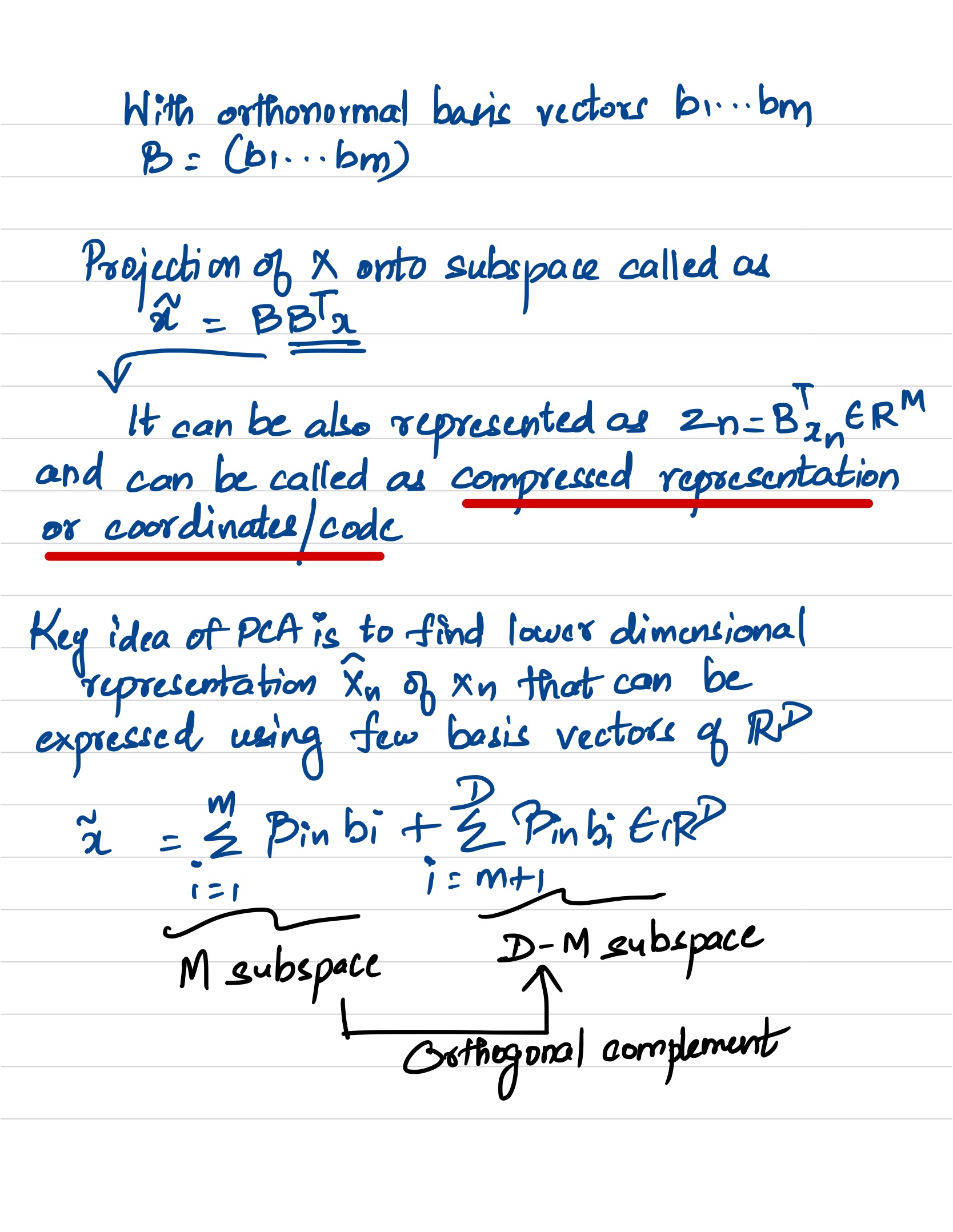
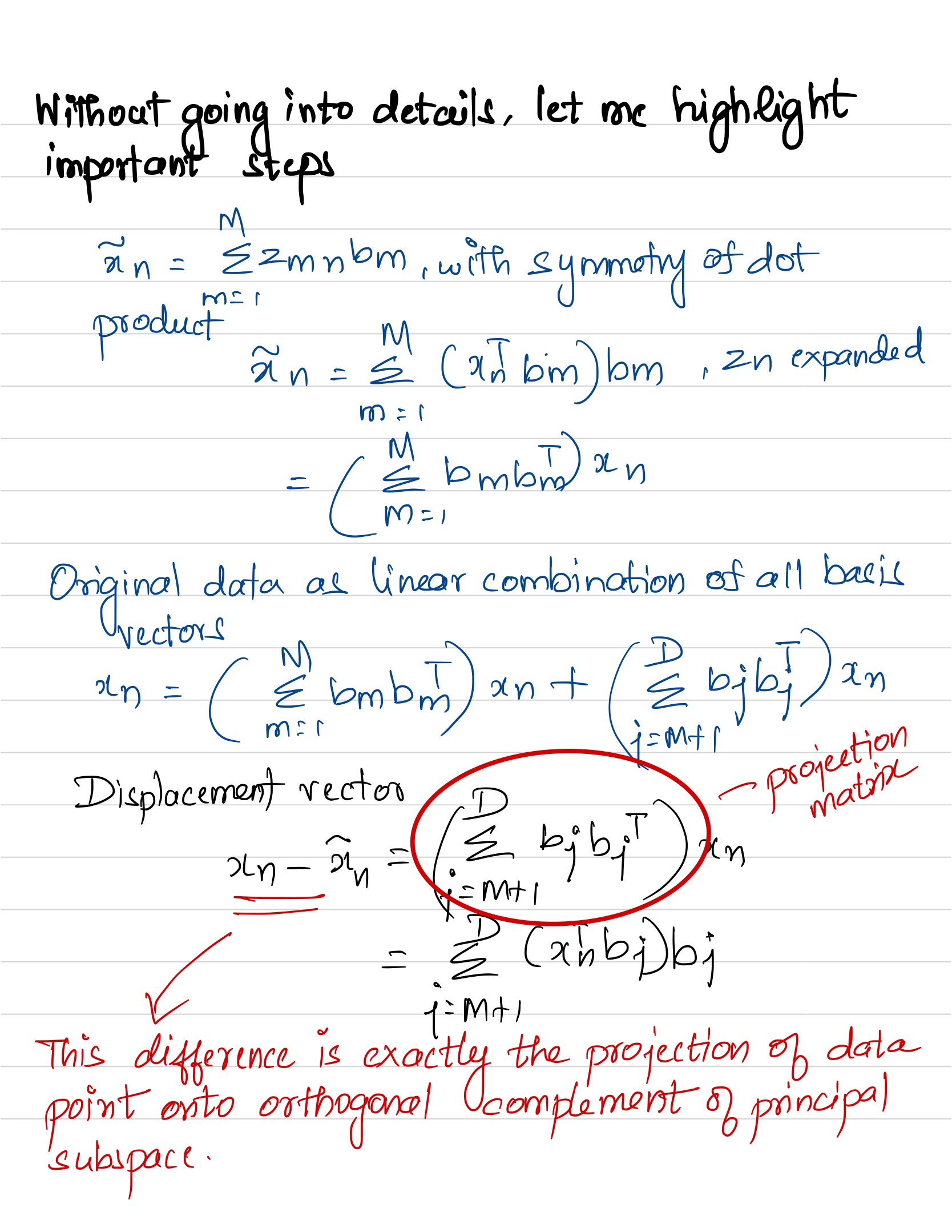
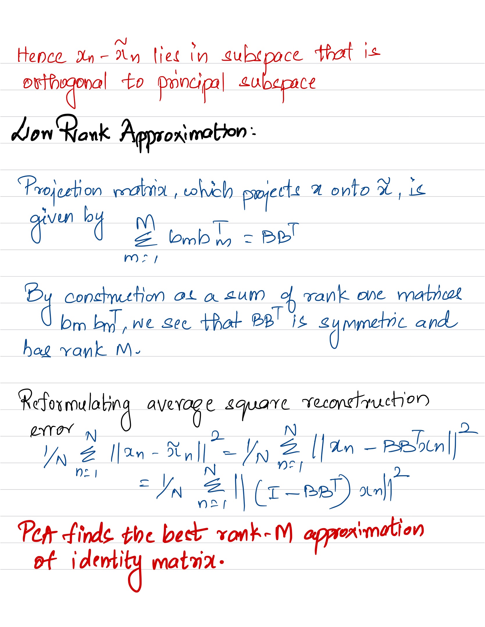
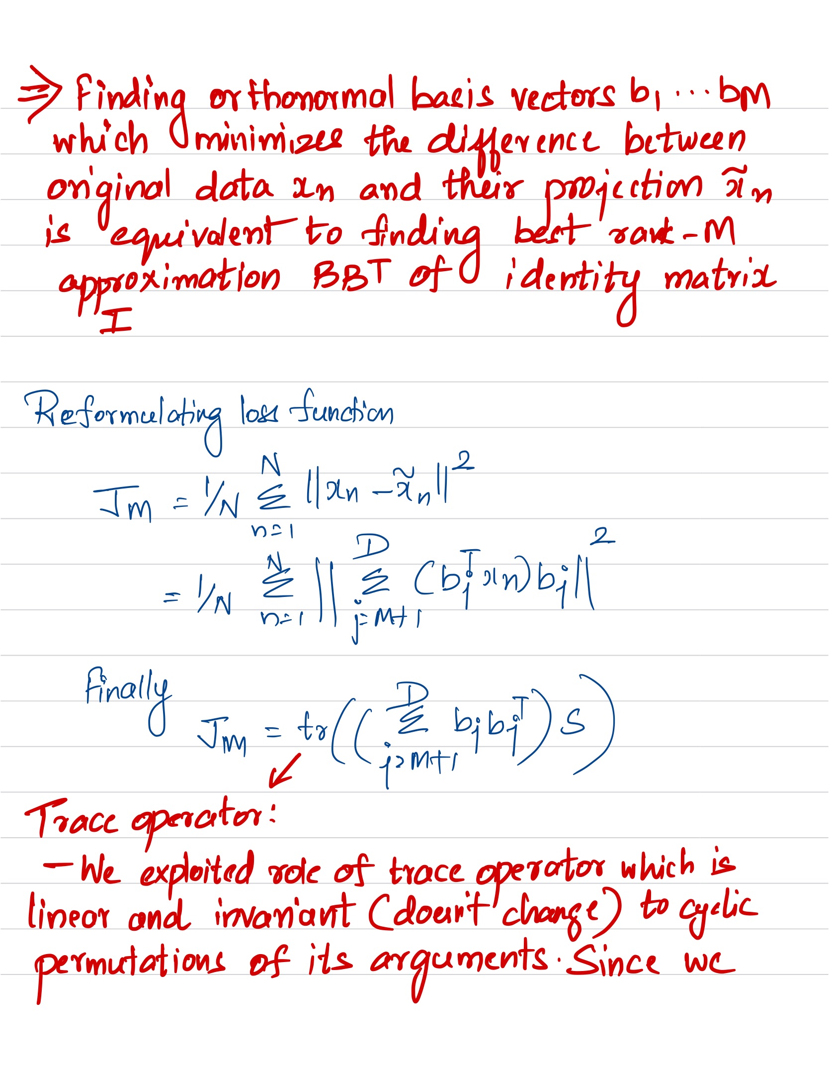
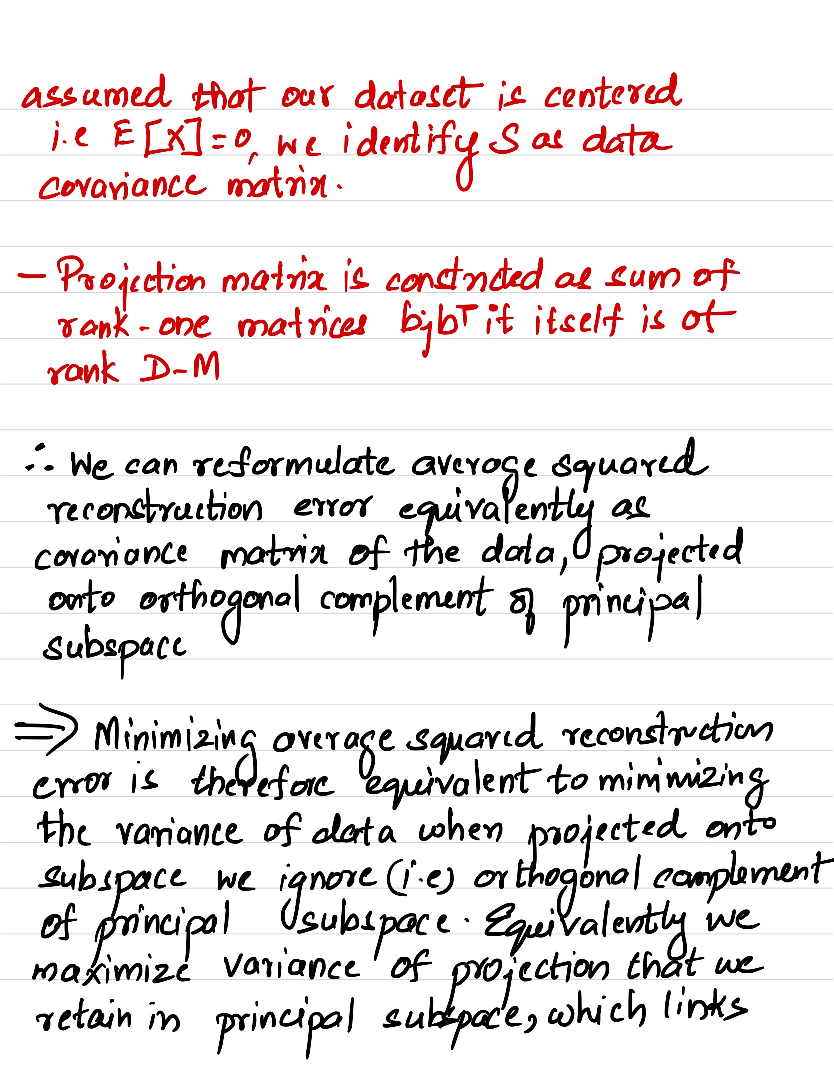
Key Steps of PCA - the below is an excerpt from MML book

The following code blocks show similar steps from my submissions.

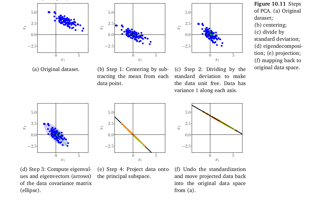
Mean subtraction We start by centering the data by computing the mean µ of the dataset and subtracting it from every single data point. This ensures that the dataset has mean 0 (Figure 10.11(b)). Mean sub- traction is not strictly necessary but reduces the risk of numerical prob- lems.
Standardization Divide the data points by the standard deviation σd of the dataset for every dimension d = 1, … , D. Now the data is unit free, and it has variance 1 along each axis, which is indicated by the two arrows in Figure 10.11(c). This step completes the standardization of the data.
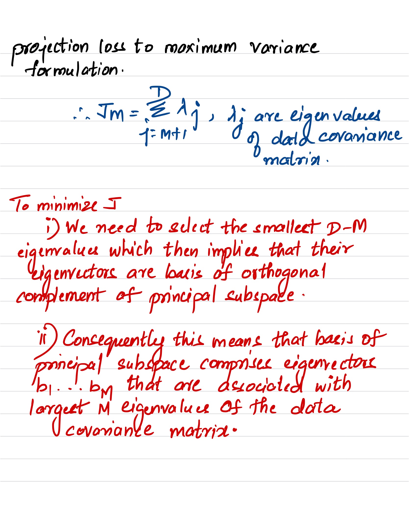
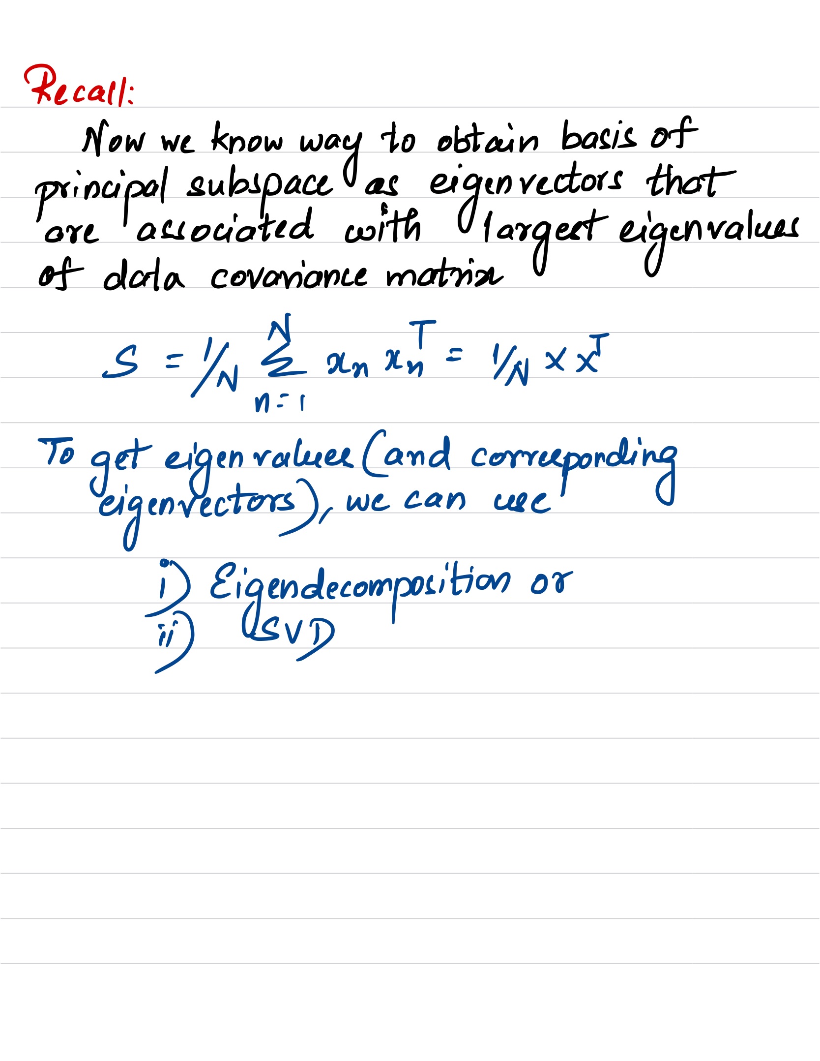
Eigendecomposition of the covariance matrix Compute the data covariance matrix and its eigenvalues and corresponding eigenvectors. Since the covariance matrix is symmetric, the spectral theorem states that we can find an ONB of . In Figure below, the eigenvectors are scaled by the magnitude of the corresponding eigenvalue. The longer vector spans the principal subspace,which we denote by U . The data covariance matrix is represented by the ellipse.
Projection We can project any data point x∗ ∈ RD onto the principal subspace: To get this right, we need to standardize x∗ using the mean µd and standard deviation σd of the training data in the dth dimension, respectively, so that

Orthogonal Projection 1D

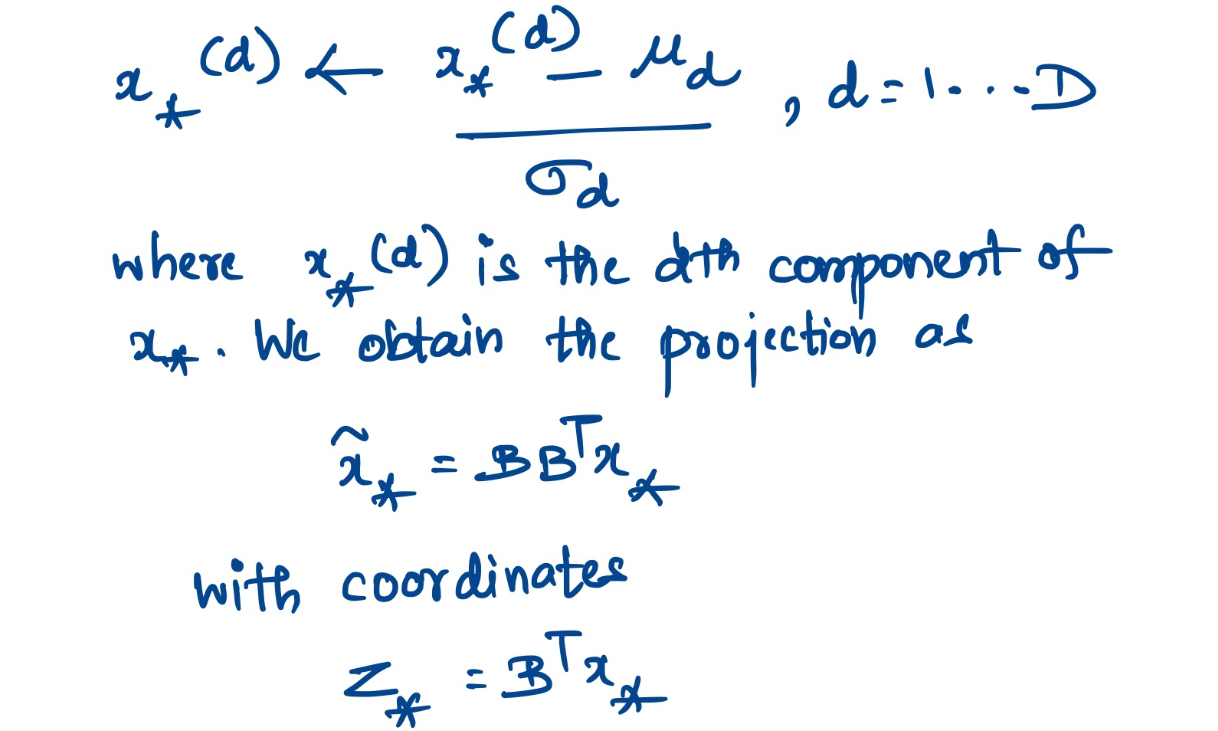
with respect to the basis of the principal subspace. Here, B is the ma- trix that contains the eigenvectors that are associated with the largest eigenvalues of the data covariance matrix as columns. PCA returns the coordinates, not the projections x∗ .

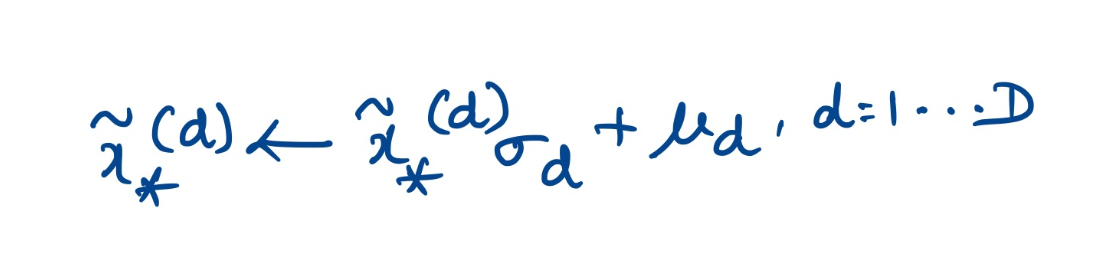
Having standardized our dataset, (10.59) only yields the projections in the context of the standardized dataset. To obtain our projection in the original data space (i.e., before standardization), we need to undo the standardization (10.58) and multiply by the standard deviation before adding the mean so that we obtain. Figure(f) below illustrates the projection in the original data space.

Orthogonal Projection 1D

Sample Code from my submissions to show orthogonal projection and key steps of PCA

Eigenface

Next, you will see what happens if you project a dataset consisting of human faces onto a subset of a basis we call the “eigenfaces”. This technique of projecting the data onto a subspace with smaller dimension, and thus reducing the number of coordinates required to represent the data, is widely used in machine learning. It can help identify trends and relationships between variables that are otherwise hidden away.

We have already prepared the eigenfaces basis using Principle Component Analysis (PCA), which finds the best possible basis to represent this smaller subspace. Next week you will derive PCA and implement the PCA algorithm, but for now you’ll simply see the results.

from sklearn.datasets import fetch_olivetti_faces
from ipywidgets import interact
%matplotlib inline
image_shape = (64, 64)
# Load faces data
dataset = fetch_olivetti_faces(data_home='./')
faces = dataset.data

Each face of the dataset is a gray scale image of size (64, 64). Let’s visualize some faces in the dataset.

plt.figure(figsize=(10,10))
plt.imshow(np.hstack(faces[:5].reshape(5,64,64)), cmap='gray');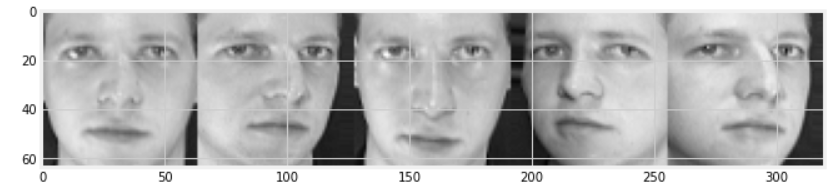

Eigen Faces

# for numerical reasons which you shall see in week 4, we normalize the dataset
mean = faces.mean(axis=0)
std = faces.std(axis=0)
faces_normalized = (faces - mean) / std

The data for the basis has been saved in a file named eigenfaces.npy, first we load it into the variable B.

B = np.load('eigenfaces.npy')[:50] # we use the first 50 basis vectors --- you should play around with this.
print("the eigenfaces have shape {}".format(B.shape))

the eigenfaces have shape (50, 64, 64) Each instance in 𝐵 is a `64x64’ image, an “eigenface”, which we determined using an algorithm called Principal Component Analysis. Let’s visualize a few of those “eigenfaces”.

plt.figure(figsize=(10,10))
plt.imshow(np.hstack(B[:5].reshape(-1, 64, 64)), cmap='gray');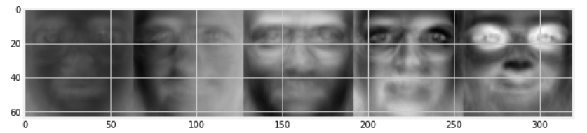

Eigen Faces

Take a look at what happens if we project our faces onto the basis 𝐵 spanned by these 50 “eigenfaces”. In order to do this, we need to reshape 𝐵 from above, which is of size (50, 64, 64), into the same shape as the matrix representing the basis as we have done earlier, which is of size (4096, 50). Here 4096 is the dimensionality of the data and 50 is the number of data points.

Then we can reuse the functions we implemented earlier to compute the projection matrix and the projection. Complete the code below to visualize the reconstructed faces that lie on the subspace spanned by the “eigenfaces”.

@interact(i=(0, 10))
def show_face_face_reconstruction(i):
    original_face = faces_normalized[i].reshape(64, 64)
    # reshape the data we loaded in variable `B` 
    B_basis = B.reshape(B.shape[0], -1).T
    face_reconstruction = project_general(faces_normalized[i], B_basis).reshape(64, 64)
    plt.figure()
    plt.imshow(np.hstack([original_face, face_reconstruction]), cmap='gray')
    plt.show()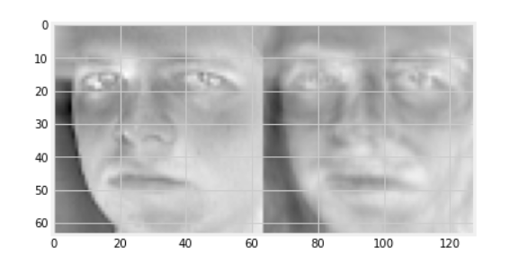

Eigen Faces

In the above you used a specially selected basis for your projections. What happens if you simply use a random basis instead?

Below, you will project the data onto 50 randomly generated basis vectors. Before you run the code cells below, can you predict the results?

B_random = np.random.randn(*B.shape)
print("the random basis has shape {}".format(B_random.shape))

the random basis has shape (50, 64, 64)

As before, we shall visualize the “faces” represented by the basis vectors.

plt.figure(figsize=(10,10))
plt.imshow(np.hstack(B_random[:5].reshape(-1, 64, 64)), cmap='gray');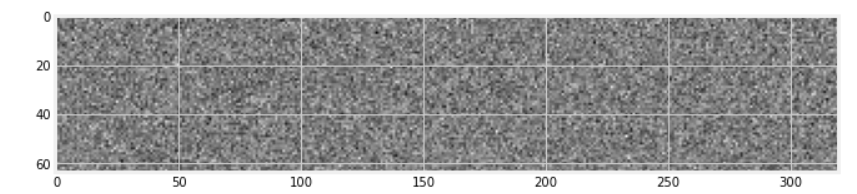

Eigen Faces

As you can see, the basis vectors do not store faces but only store random noise.

Let us now try to project the faces onto this basis.

@interact(i=(0, 10))
def show_face_face_reconstruction(i):
    original_face = faces_normalized[i].reshape(64, 64)
    # reshape the data we loaded in variable `B` 
    B_basis = B_random.reshape(B_random.shape[0], -1).T
    face_reconstruction = project_general(faces_normalized[i], B_basis).reshape(64, 64)
    plt.figure()
    plt.imshow(np.hstack([original_face, face_reconstruction]), cmap='gray')
    plt.show()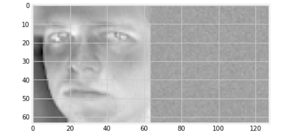

Eigen Faces

You can see how important it is to use a technique like PCA when selecting your basis for projection!

PCA Submission notebooks

Refer to Gitlab (TO-DO, replace with link)

References

There are other commonly searched, high page ranked sources for PCA algorithm which are not limited to the following

Essence of Linear Algebra using 100+ years old PCA

#Essence of Linear Algebra using 100+ years old PCA (Principal Component Analysis)

#Unveiling Hidden Patterns: Principal Component Analysis (PCA)

#Here’s a breakdown of the key concepts:

#Why Use SVD for PCA?

#Beyond Euclidean Distance: Kernel PCA for Non-Linear Relationships

#Probabilistic PCA (PPCA): A Latent Variable Approach to Dimensionality Reduction

#Latent Variables: The Underlying Structure

#The Generative Model of PPCA:

#PPCA vs. PCA: Key Differences

#Key Steps of PCA - the below is an excerpt from MML book

#Sample Code from my submissions to show orthogonal projection and key steps of PCA

#Eigenface

#PCA Submission notebooks

#References

Related Posts

Essence of Linear Algebra using 100+ years old PCA (Principal Component Analysis)

Unveiling Hidden Patterns: Principal Component Analysis (PCA)

Here’s a breakdown of the key concepts:

Why Use SVD for PCA?

Beyond Euclidean Distance: Kernel PCA for Non-Linear Relationships

Probabilistic PCA (PPCA): A Latent Variable Approach to Dimensionality Reduction

Latent Variables: The Underlying Structure

The Generative Model of PPCA:

PPCA vs. PCA: Key Differences

Key Steps of PCA - the below is an excerpt from MML book

Sample Code from my submissions to show orthogonal projection and key steps of PCA

Eigenface

PCA Submission notebooks

References