Neural Networks is beautiful

#Objectives

This blog post was born to appreciate the power and beauty of Neural Networks in my view. This post is a good next post to read after reading my Essence of Calculus and Maximum Likelihood, Probability posts.

• This post serves my own reference materials and it contains some of the basic flows, concepts which repeats itself in same form or different forms in advanced Neural Network topics.
• This post will be referred in future blog posts as well.

#Intuition

Let me rephrase the importance of non-linear separation of data points in certain problems.

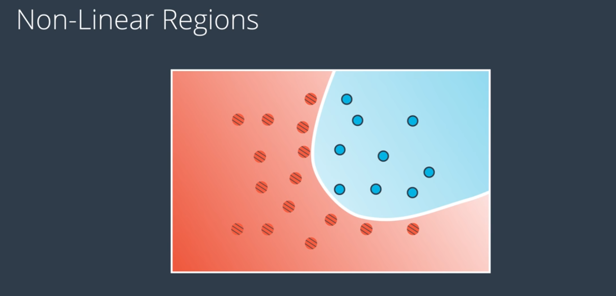
In nutshell, for the data which is not separable with line, we are going to create a probability function, where points in blue region are more likely to be blue and points in red region are more likely to be red. Curve which separates them is set of points which are set of points which are equally likely to be red or blue.

#Flow

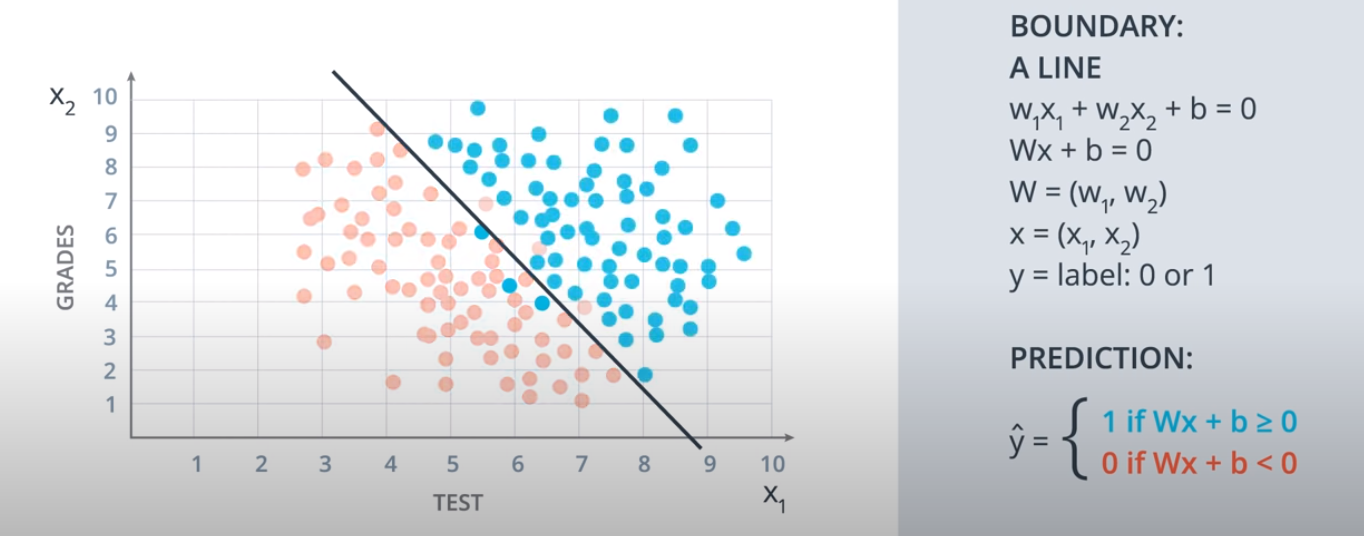
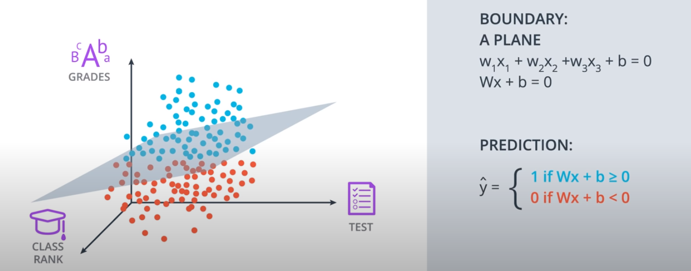
• From idea of linear separation of data starting from two dimensional line to three dimensional plane to n-dimensional.
• Remember, linear combination is still linear. So the above said linear separation embedded into Perceptron (see below), can still be linear without a non-linear activation.
• Next step is beauty of Perceptron algorithm (a.k.a trick), followed by combination of Perceptrons which leads to beautiful Neural Networks which creates the necessary non-linear boundary to separate the data points.

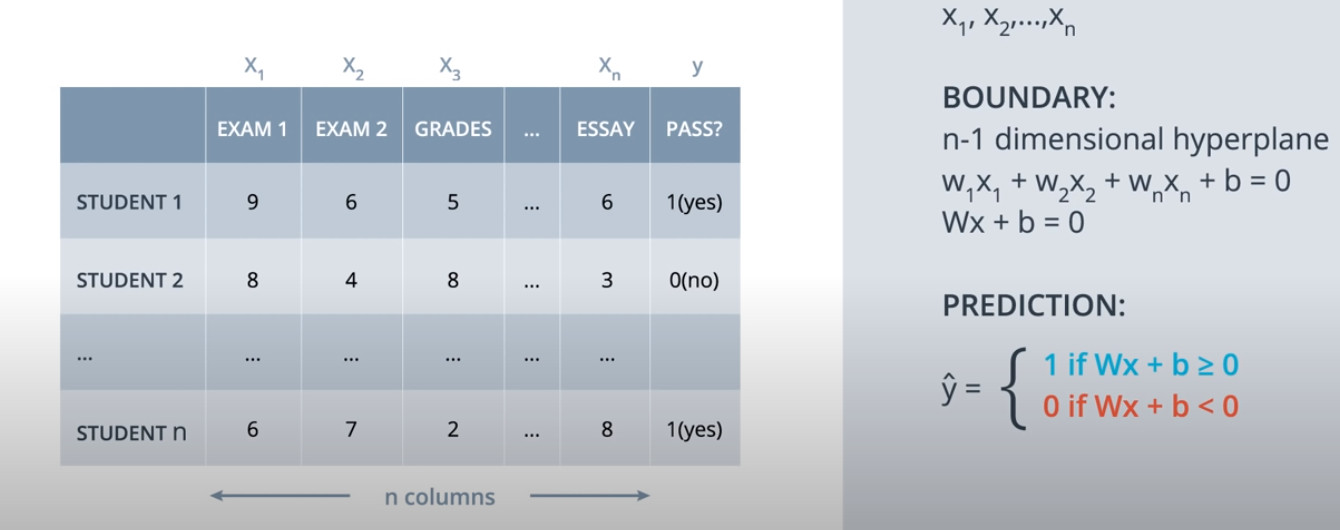
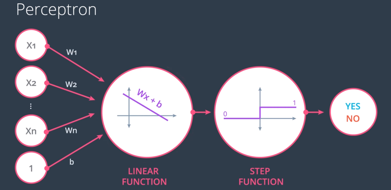
#Perceptron

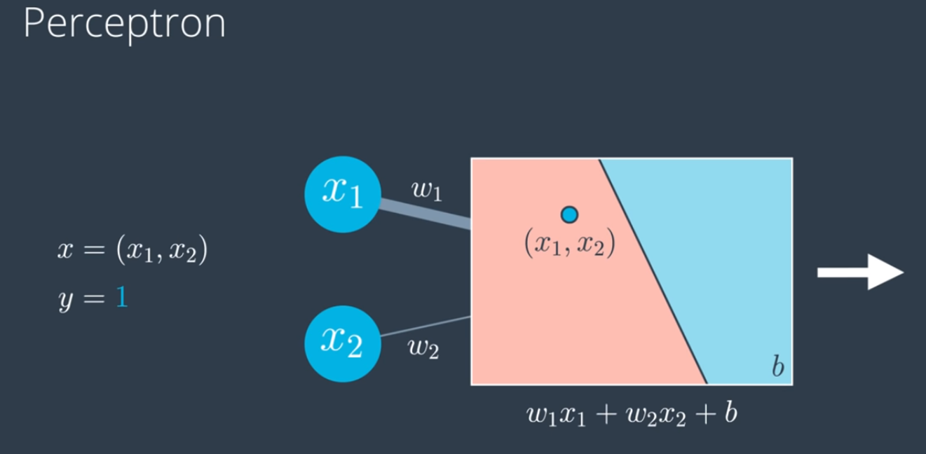
• A perceptron is a major building block of neural networks. Perceptrons are graphs that have nodes and edges.

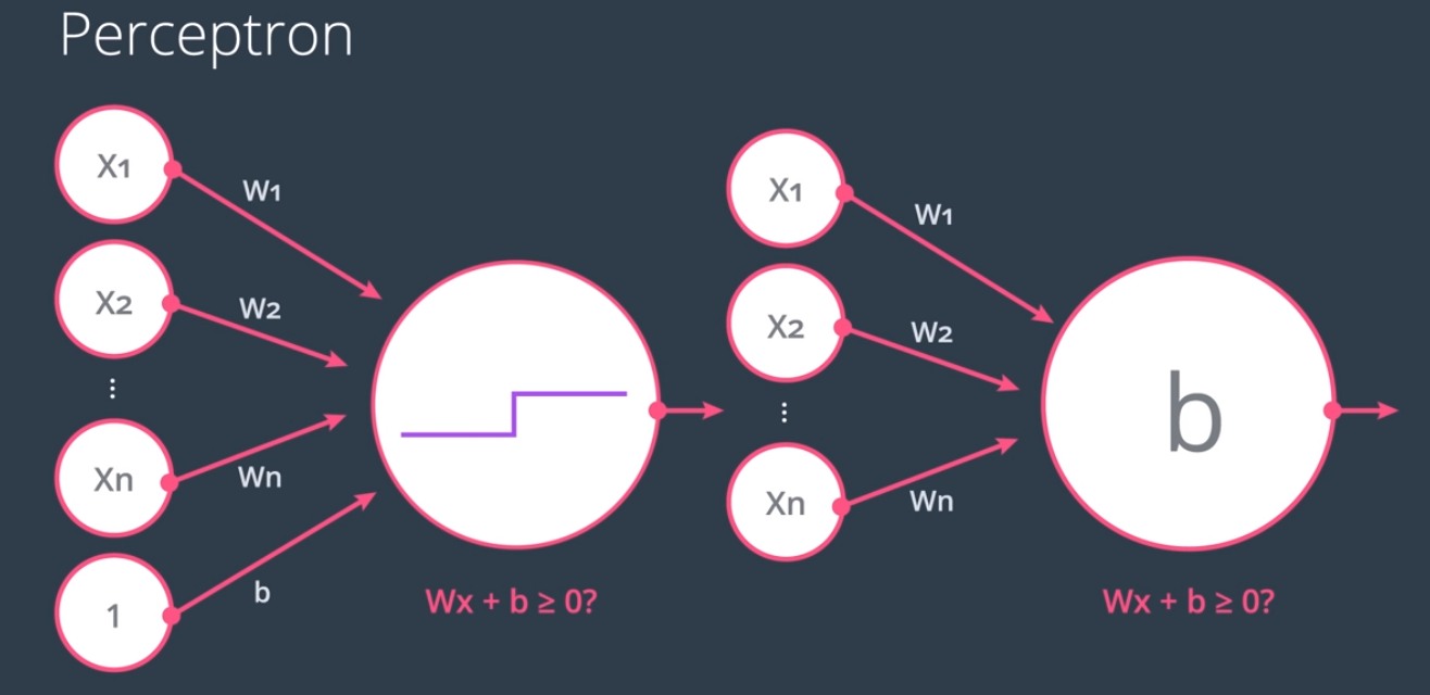
• One another way to represent bias

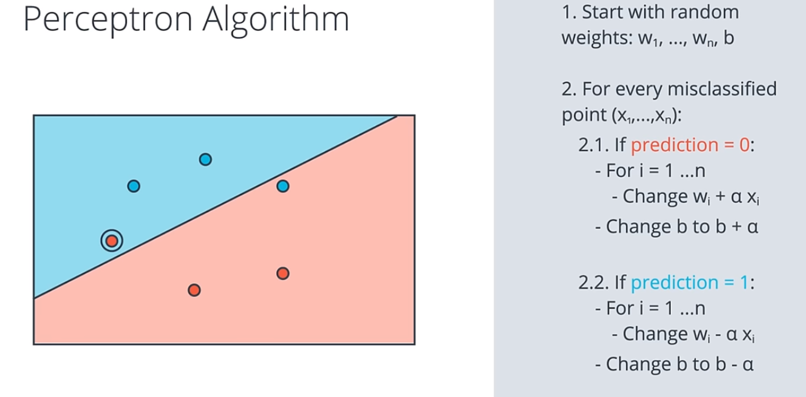
Perceptron trick or algorithm, for only and all misclassified points, it tries to move the separation close or rather away from the individual data points.

#Importance

#Activation Functions

I will scratch the surface and re-iterate the importance of activation functions. In this post, I will not go in depth on formulas of different activation funcion. Please refer to the linked posts from the beginning of this post.

| The fact that a linear function of a linear function is itself a linear function. So having multiple layers in a neural network doesn’t let the neural network compute any more complex features or learn anything more complex than just a linear function. So in the general case, if you have a neural network with multiple layers and you were to use a linear activation function for all of the hidden layers and also use a linear activation function for the output layer, then it turns out this model will compute an output that is completely equivalent to linear regression

• A more general function that introduces non-linearity into a neural network.

• Non-linearity is crucial for neural networks to learn complex patterns in data.

• Activation functions take an input from a neuron (a weighted sum of its previous layer’s outputs) and apply a mathematical function to it, producing the output that gets sent to the next layer.

• Relu —> if output can only take on non-negative values, such as if you’re predicting the price of a house, that can never be negative, then the most natural choice will be the ReLU activation function because as you see here, this activation function only takes on non-negative values, either zero or positive values

• Hidden layers of a neural network —> It turns out that the ReLU activation function is by far the most common choice in how neural networks are trained by many practitioners today.

• If you compare the ReLU and the sigmoid activation functions, the ReLU is a bit faster to compute because it just requires computing max of 0, z, whereas the sigmoid requires taking an exponentiation and then a inverse and so on, and so it’s a little bit less efficient. But the second reason which turns out to be even more important is that the ReLU function goes flat only in one part of the graph; whereas the sigmoid activation function, it goes flat in two places.

• If you’re using gradient descent to train a neural network, then when you have a function that is flat in a lot of places, gradient descents would be really slow. Small gradients —> slow learning (in context of Gradient Descent).s

• Researchers have found that using the ReLU activation function can cause your neural network to learn a bit faster as well, which is why for most practitioners if you’re trying to decide what activation functions to use with hidden layer, the ReLU activation

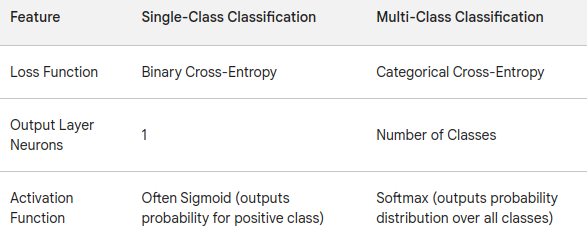
• To summarize, for the output layer, use a sigmoid, if you have a binary classification problem; linear, if y is a number that can take on positive or negative values, or use ReLU if y can take on only positive values or zero positive values or non-negative values. Softmax for multi-class classification. Then for the hidden layers I would recommend just using ReLU as a default activation function.

• Sometimes LeakyReLU activation function works a little bit better than the ReLU activation function.

• Sometimes Hyperbolic Tangent, where the output ranges between minus one and one. The derivatives are larger which makes an impact on Neural Networks training.

Before we go to next section, recall jargons

• Loss: The error for a single data point (sample)
• Cost: The loss for the entire dataset, which is the sum of losses on individual training samples
• Error: The difference between the actual and predicted values

#Error Functions

—> To apply Gradient descent and for effective learning process, it is important to choose error functions which should be differentiable and continous

One approach to reducing errors might be to simply count the number of errors and then make changes until the number of errors is reduced. But taking a discrete approach like this can be problematic—for example, we could change our line in a way that gets closer to the solution, but this change might not (by itself) improve the number of misclassified points.

Instead, we need to construct an error function that is continuous. That way, we can always tell if a small change in the line gets us closer to the solution. We’ll do that using the log-loss error function. Generally speaking, the log-loss function will assign a large penalty to incorrectly classified points and small penalties to correctly classified points. For a point that is misclassified, the penalty is roughly the distance from the boundary to the point. For a point that is correctly classified, the penalty is almost zero.

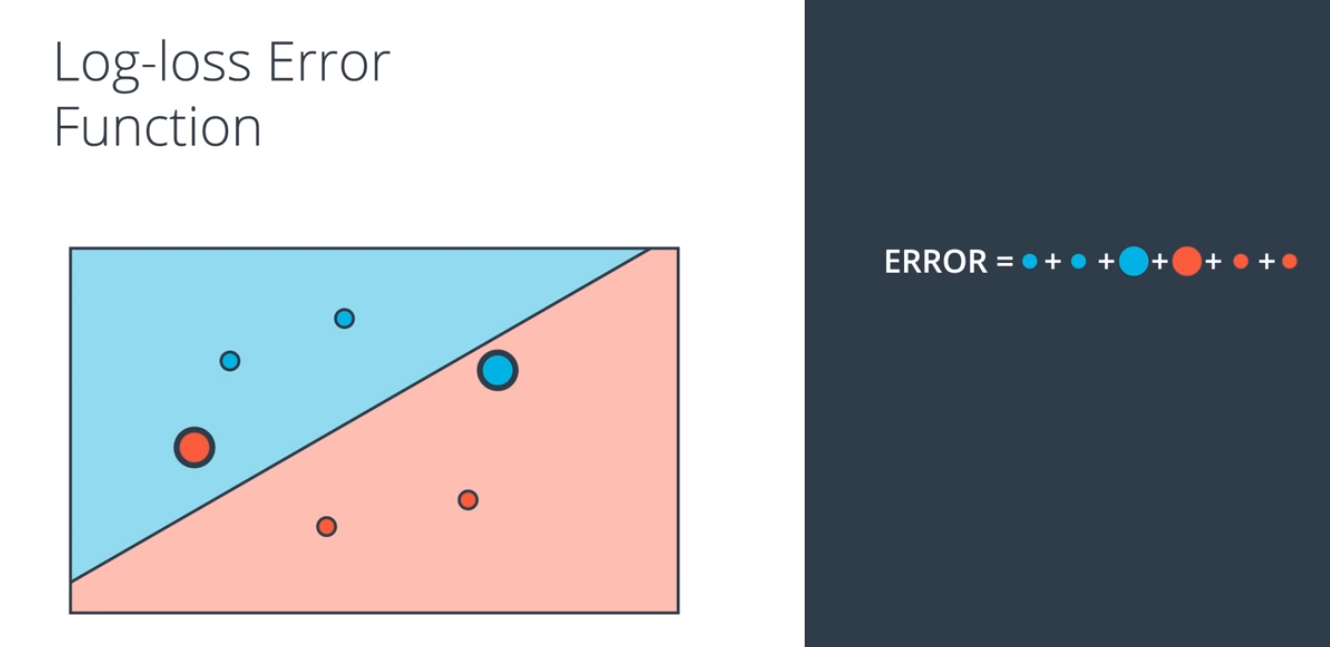
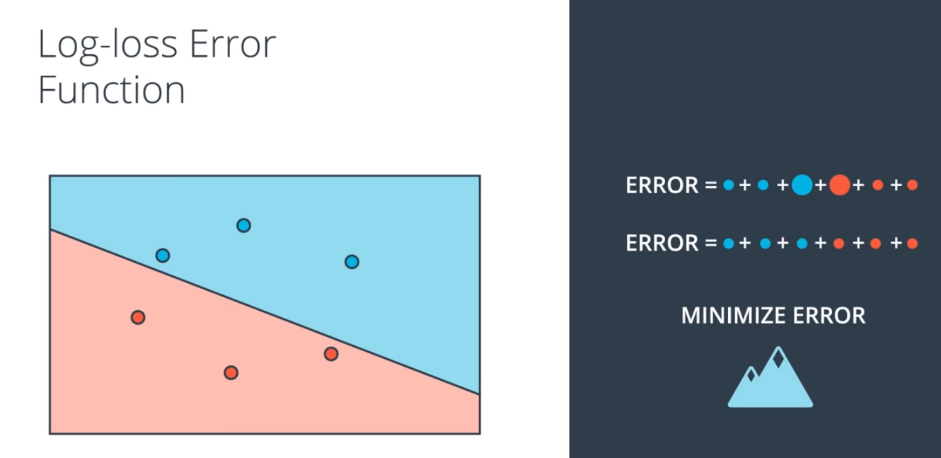
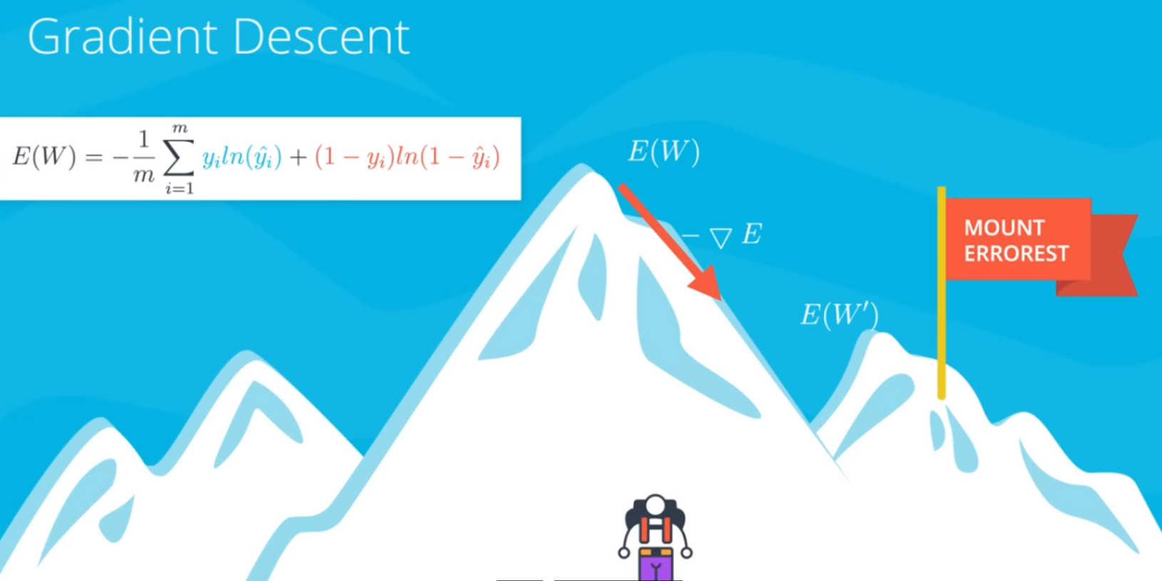
We can then calculate a total error by adding all the errors from the corresponding points. Then we can use gradient descent to solve the problem, making very tiny changes to the parameters of the line in order to decrease the total error until we have reached an acceptable minimum.

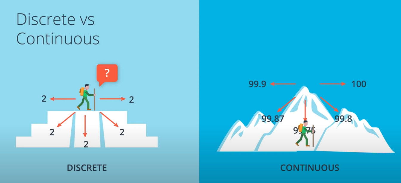
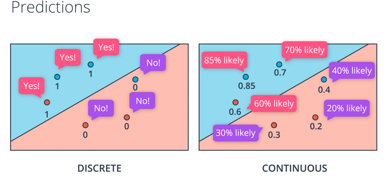
The prediction is essentially the answer we get from the algorithm:

• A discrete answer will be of the form “no” or “yes” (or 0 or 1).
• A continuous answer will be a number, normally between 0 and 1.
• When our prediction gives us a continuous number between 0 and 1, this is equivalent to the probability that the given data point should belong to the given classification (e.g., a data point might get a prediction of 0.5, with this being equivalent to a 50% probability that it is correctly classified).

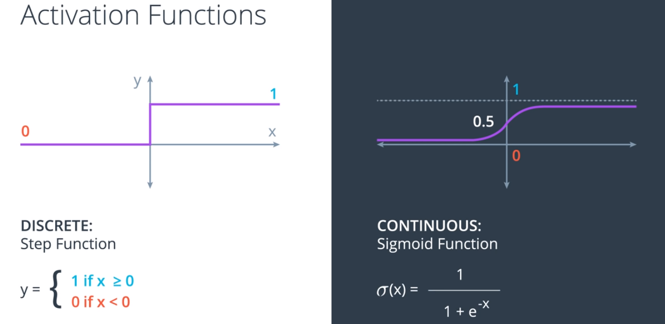
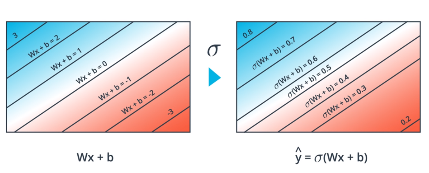
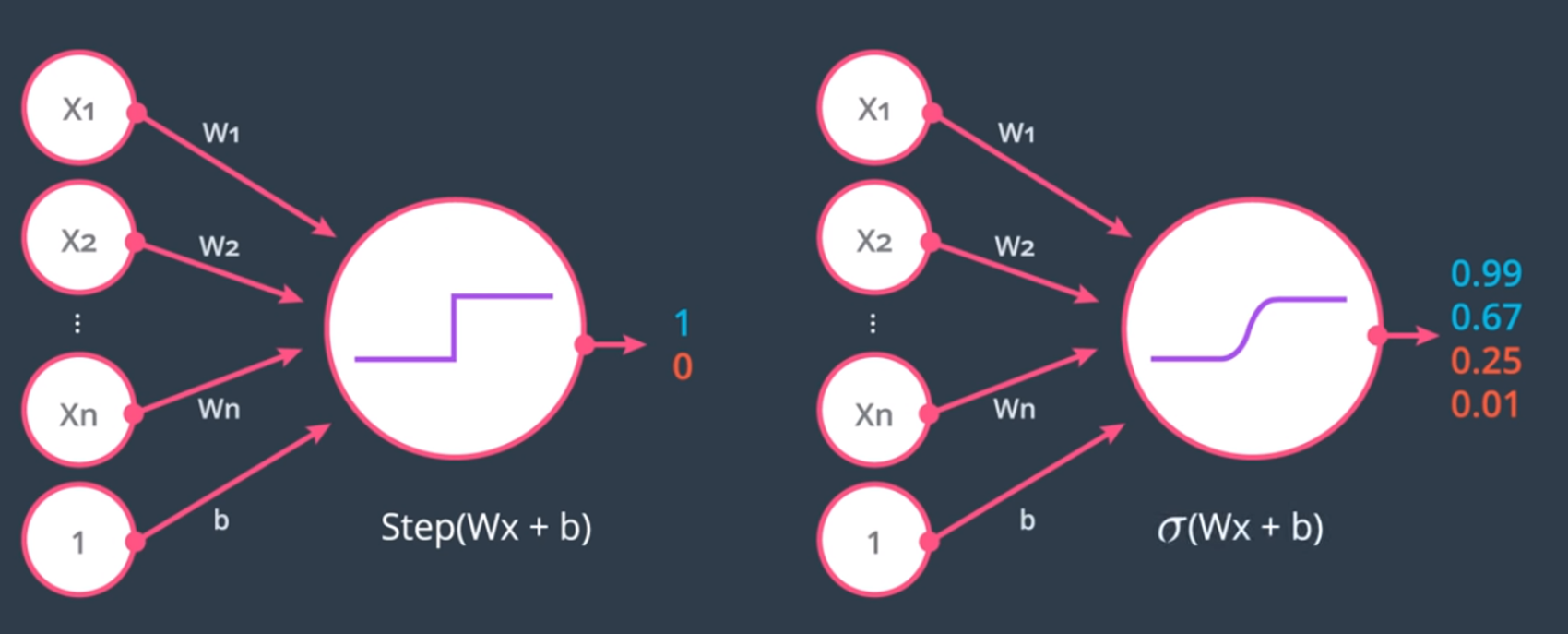
One way we move from discrete predictions to continuous is to simply change our activation function from a step function to a sigmoid function. A sigmoid function is an s-shaped function that gives us:

• Output values close to 1 when the input is a large positive number
• Output values close to 0 when the input is a large negative number
• Output values close to 0.5 when the input is close to zero

With our linear example, the probability is a function of the distance from the line. The further a data point is from the line, the larger the probability that it is classified correctly.

#Cross-Entropy

Now we know the way of looking at individual outputs as probabilities.

• Refer to my probability post on maximum likelihood and related topics. In the beginning of this post, I have referred to the related posts.

One method we can use for this is called maximum likelihood. In this approach, we pick the model that gives the existing labels in our historical data (which we know are correct) the highest probability.

The key idea is that we want to calculate P(all), which is the product of all the independent probabilities of each point. This helps indicate how well the model performs in classifying all the points. To get the best model, we will want to maximize this probability.

Our aim here was to give you a general intuition for why we would want to get the maximum likelihood.

Product to sum —> I am not going to go deep on this. Our old friend Logarithms comes into picture.

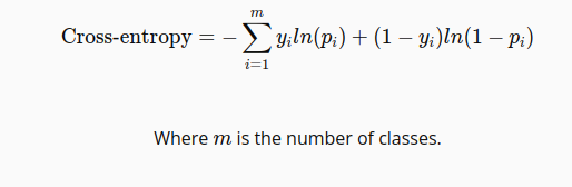
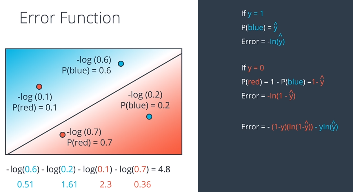
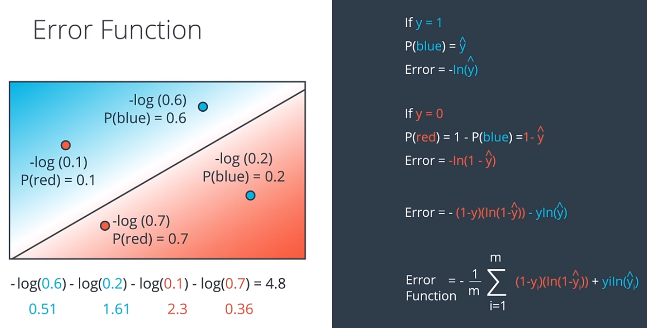
• The logarithm of a number between zero and one is always a negative number, so that means all of our probabilities (which are between zero and one) will give us negative results when we take their logarithm. Here comes cross entropy, sum of negative logarithms of our probabilities.

A good model gives a high probability and the negative of a logarithm of a large number is a small number—thus, in the end:

• A high cross-entropy indicates a bad model
• A low cross-entropy indicates a good model

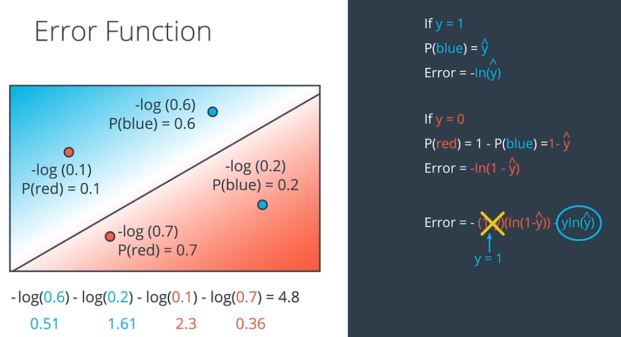
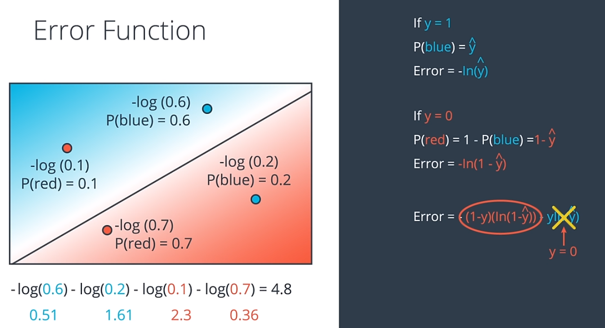
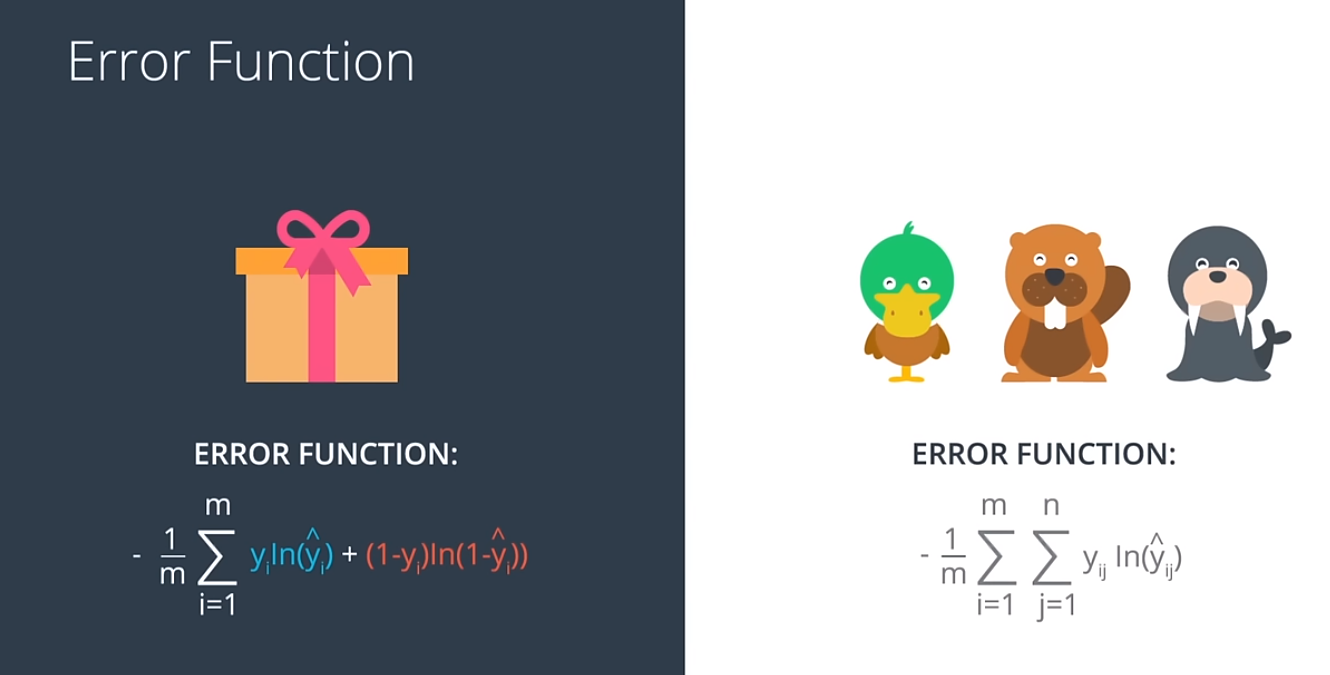
We can think of the negatives of these logarithms as errors at each point. The higher the probability, the lower the error—and the lower the cross-entropy. So now our goal has shifted from maximizing the probability to minimizing the cross-entropy.

Cross entropy essentially says, “If I have a bunch of events and a bunch of probabilities, how likely is it that those events happen based on the probabilities?”

• If it’s likely, then we have a small cross-entropy.
• If it’s unlikely, then we have a large cross-entropy.

#Cross entropy (specific log loss) + Logistic Regression

#Minimize Error Function

Now, we can go to the next step of reducing the error function. So far the flow is data, random model with right activation functions to error functions to minimizing error functions using Gradient descent or other methods.

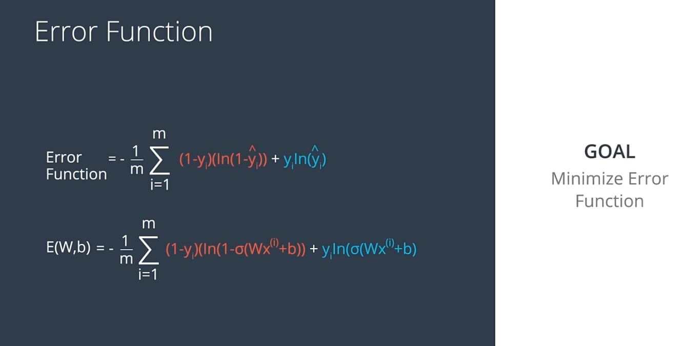
Multi cross entropy for multiple classes.

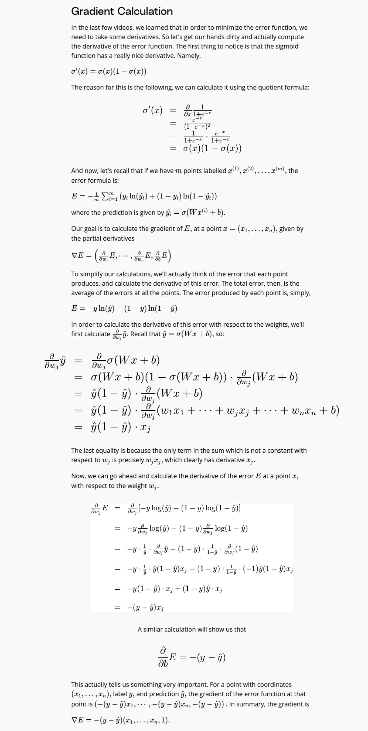
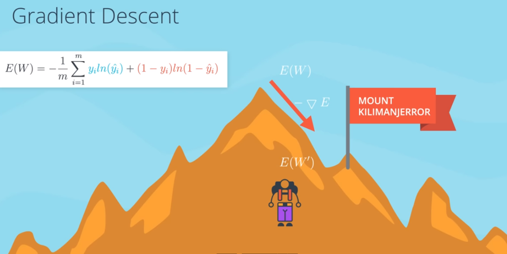
#Gradient Descent

• Please refer to my calculus post on more math notes. However, in this post, I am going to keep it light weight.

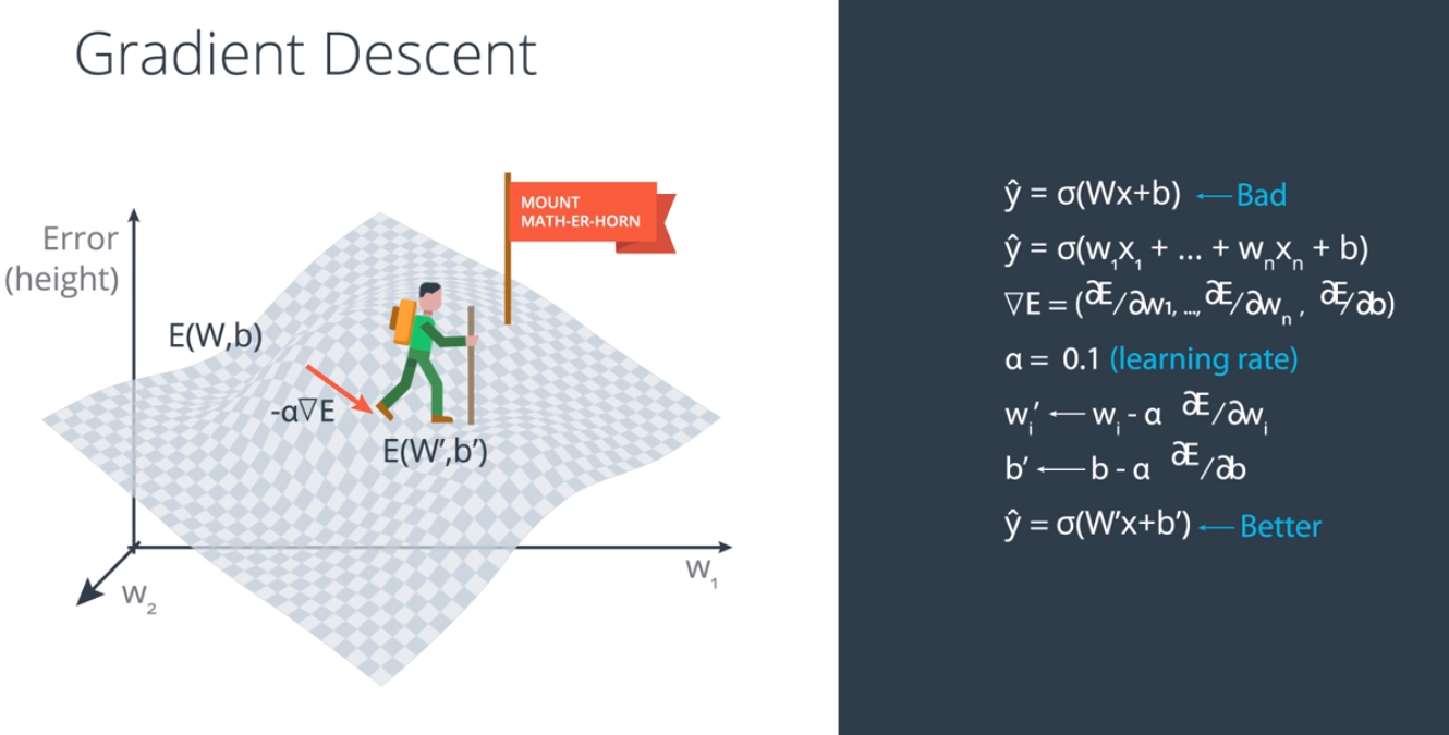
Gradient Descent Psedocode and programmatic intuition

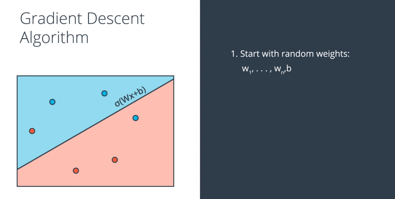
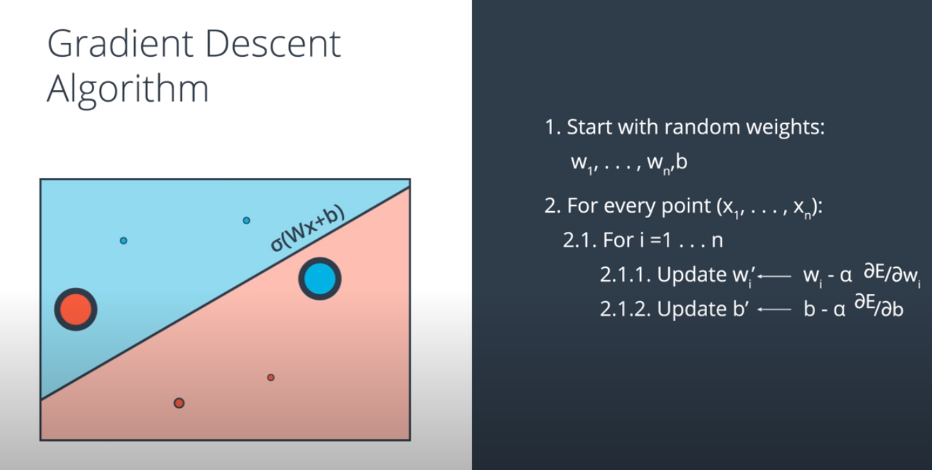
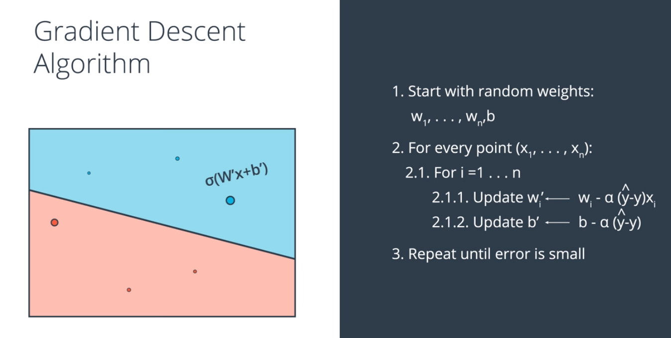
Please also refer to my notes and code at My Gitlab Page and Code

Both Perceptron trick and Gradient descent, the point which is misclassified tells the boundary to comes closer. However, if point is correctly classified, in Gradient descent, the point is telling the boundary line to go farther away but Perceptron trick does nothing. Interesting.

#Neural Network Architecture

Finally, after knowing the importance of non-linear activations, we can dive into Neural Network architecture, which is powerful, beutiful and one of the best inventions.

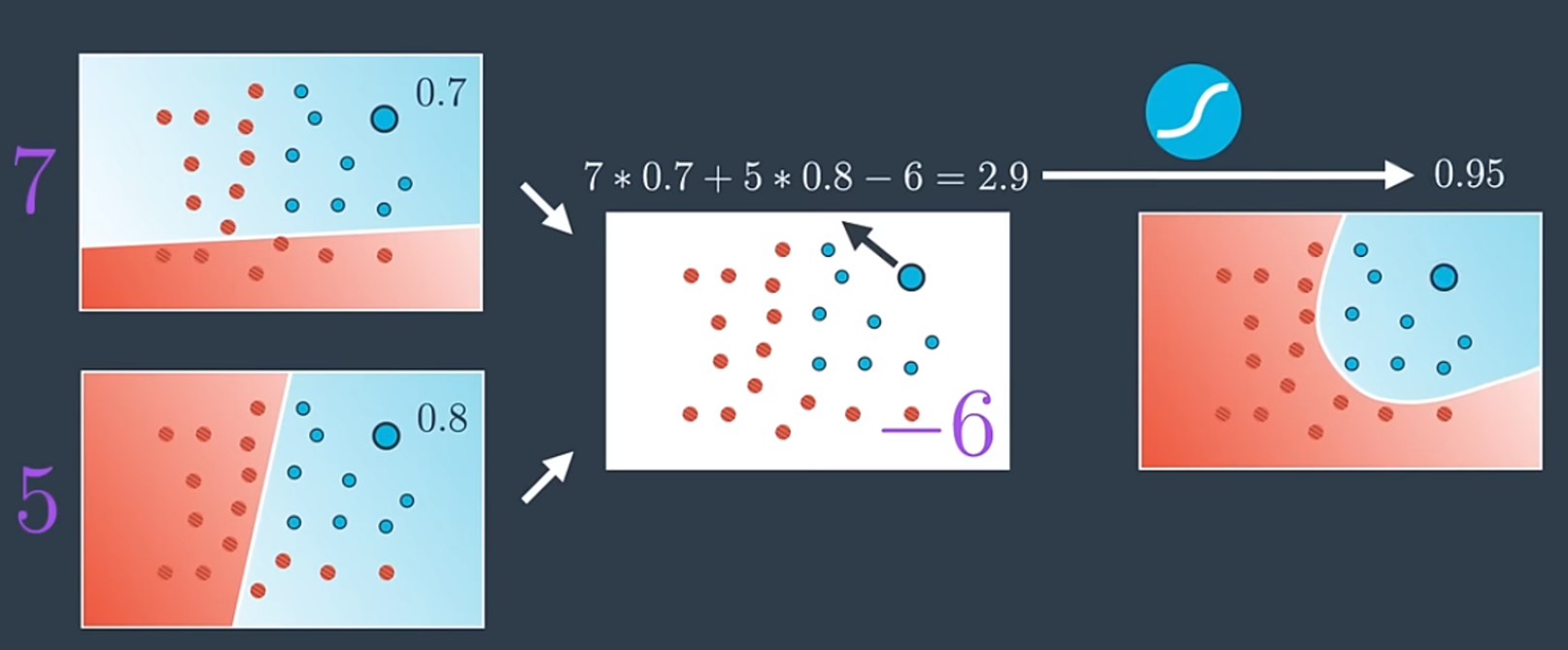
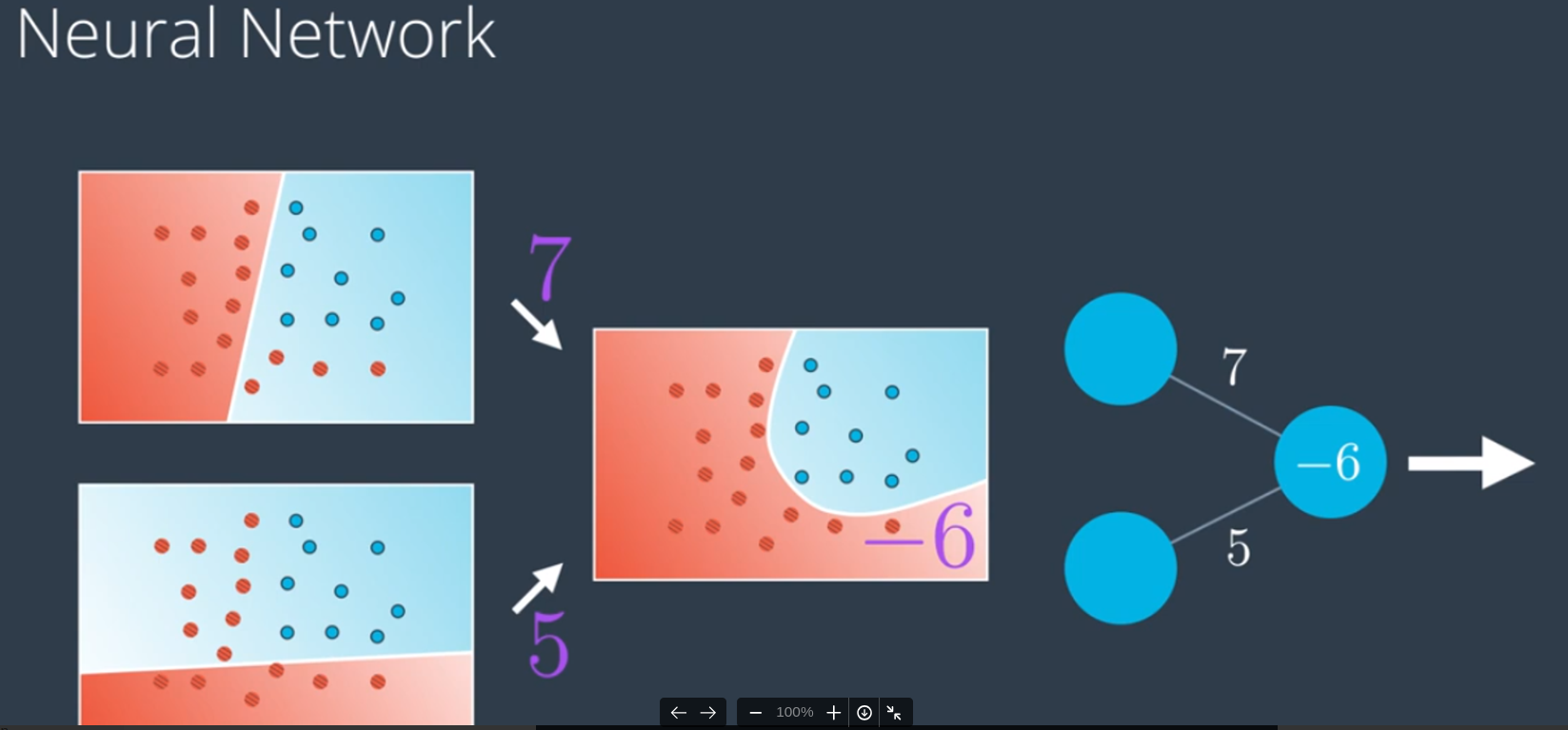
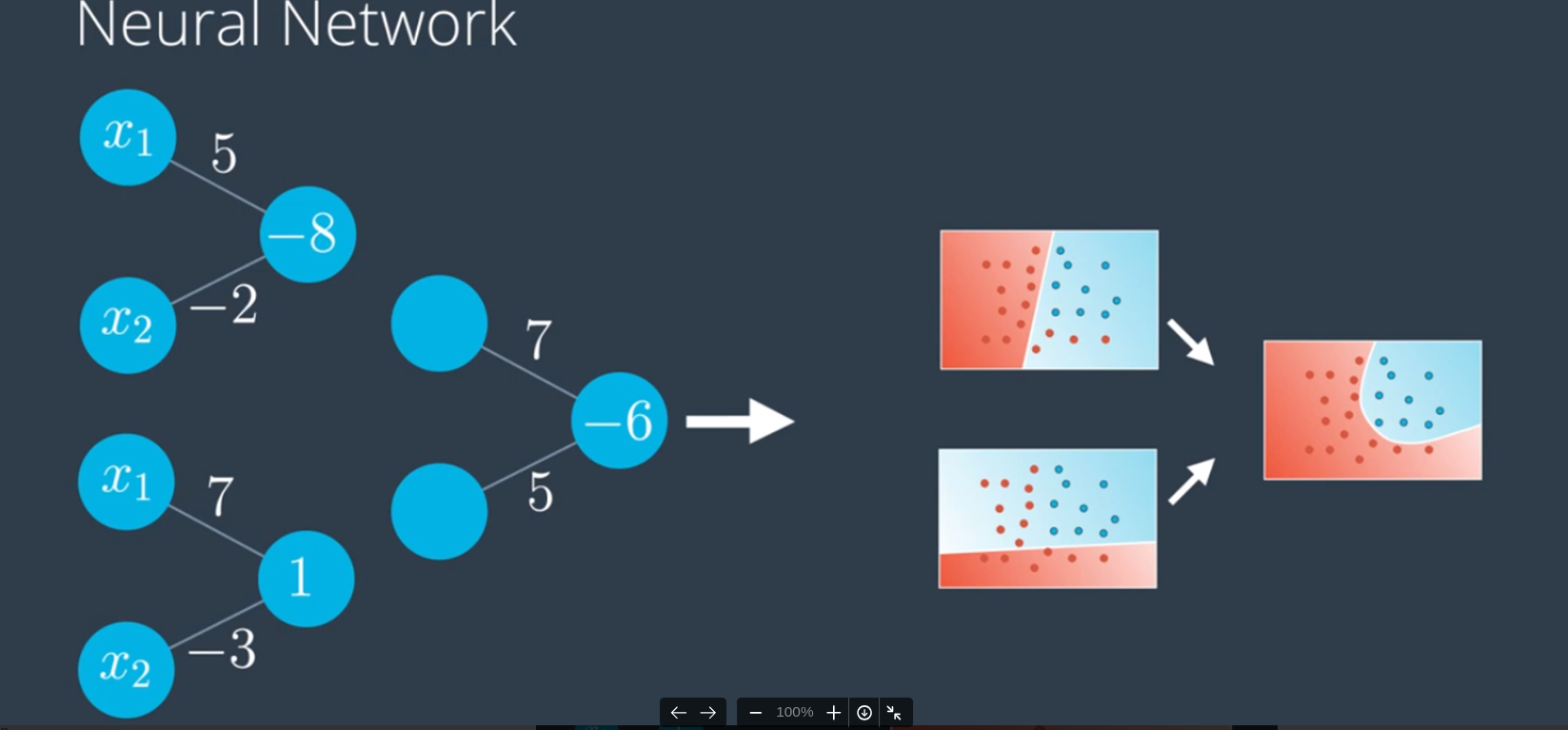
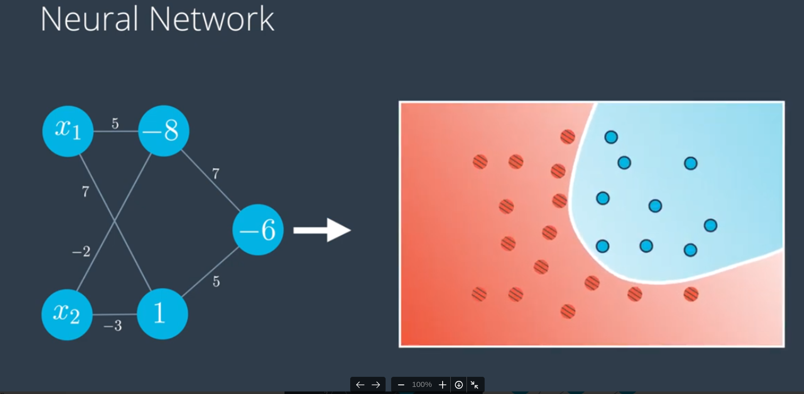
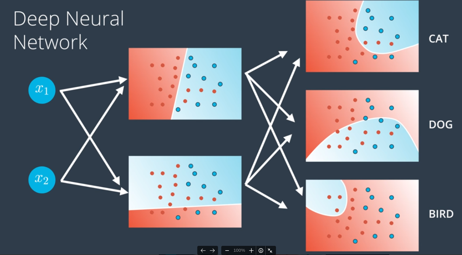
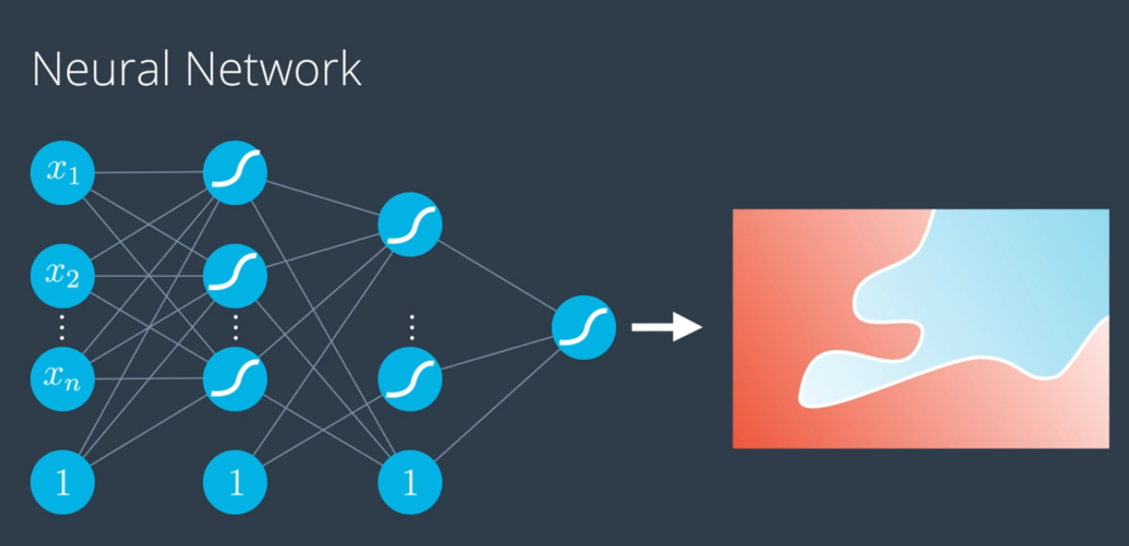
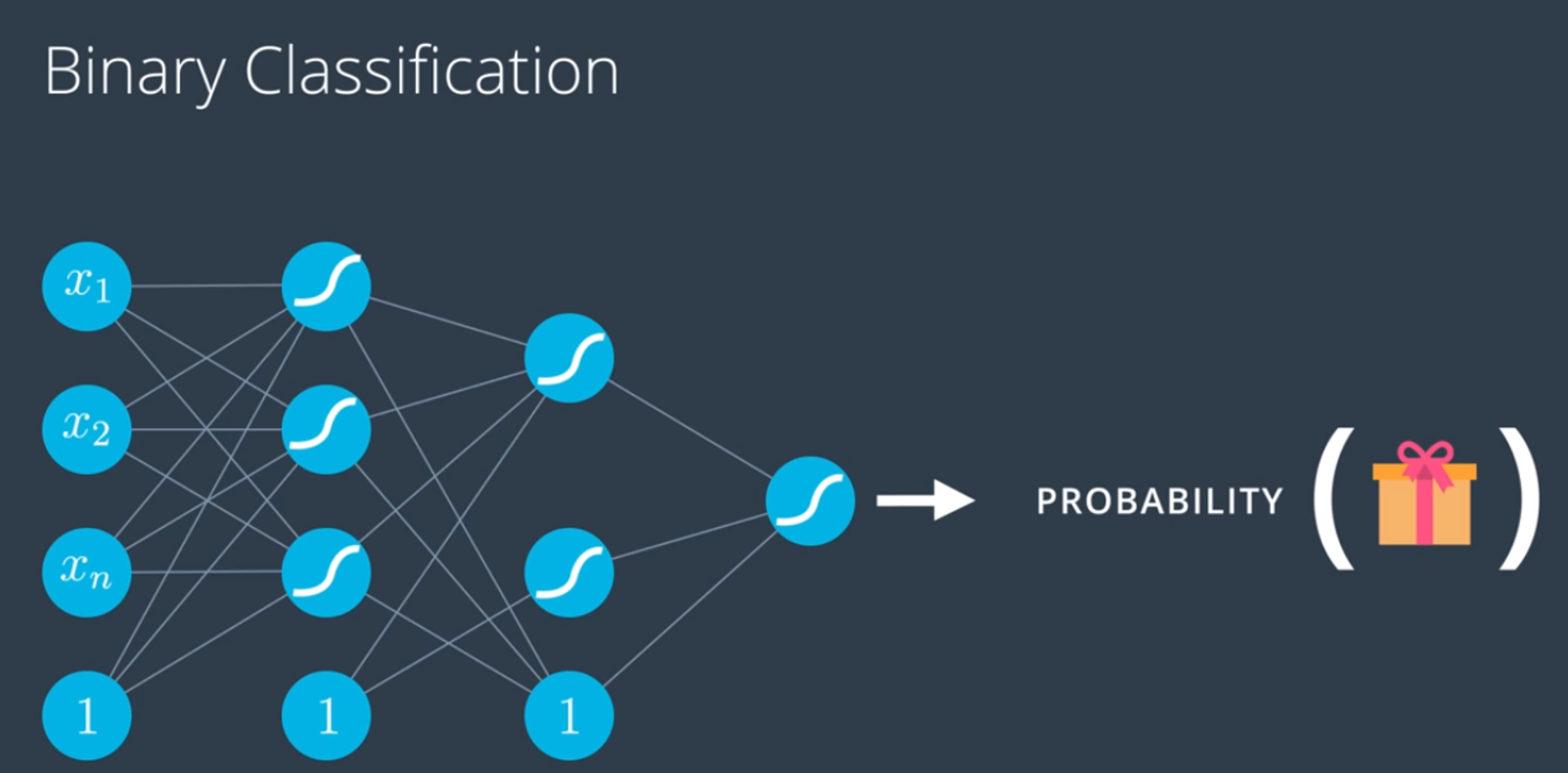
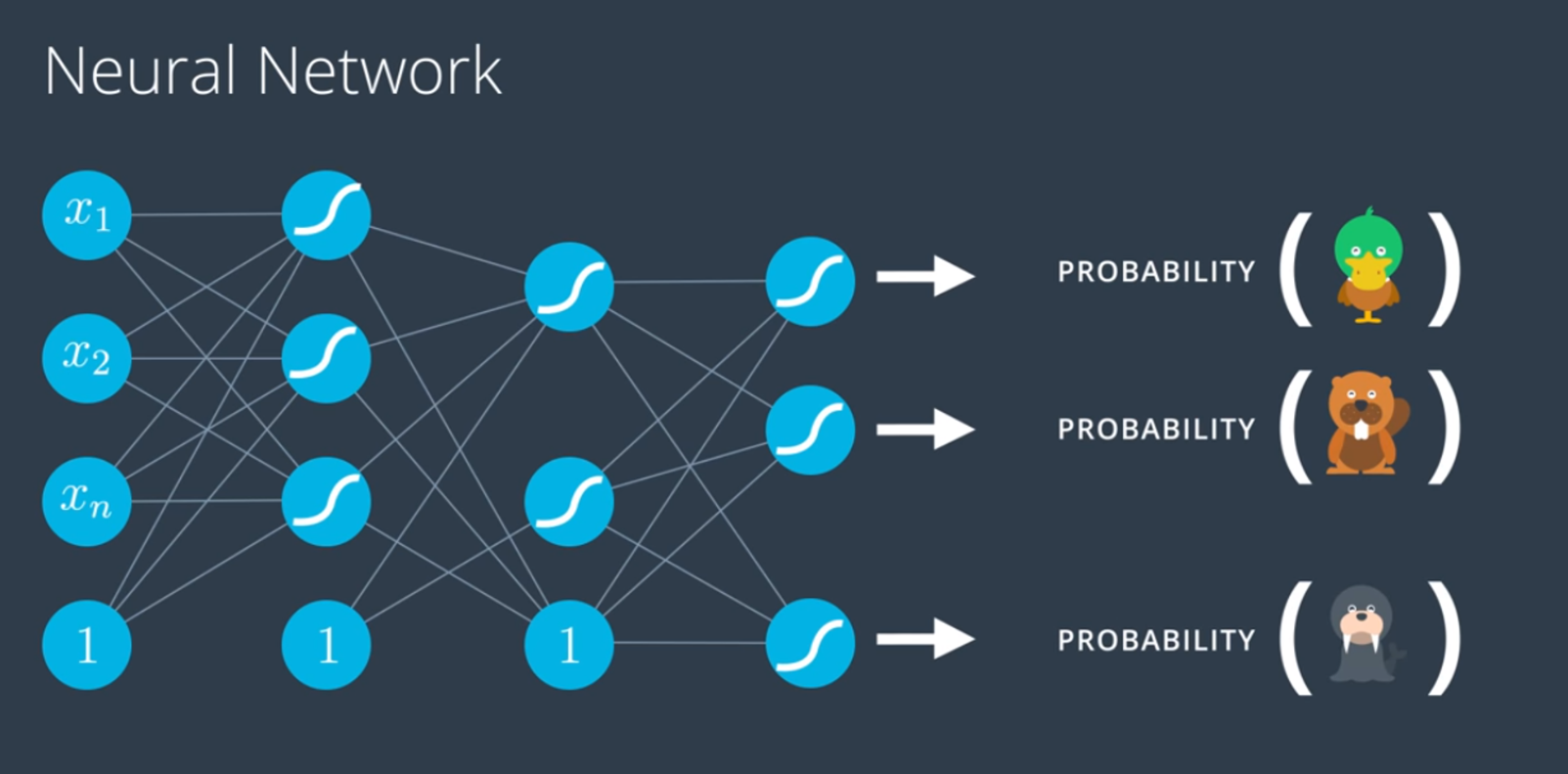
I am going to let the pictures talk millions of words rather than just words. The idea is to share my notes in effective way for revising and motivate to study complex Neural Network architectures which are coming next in my other posts.

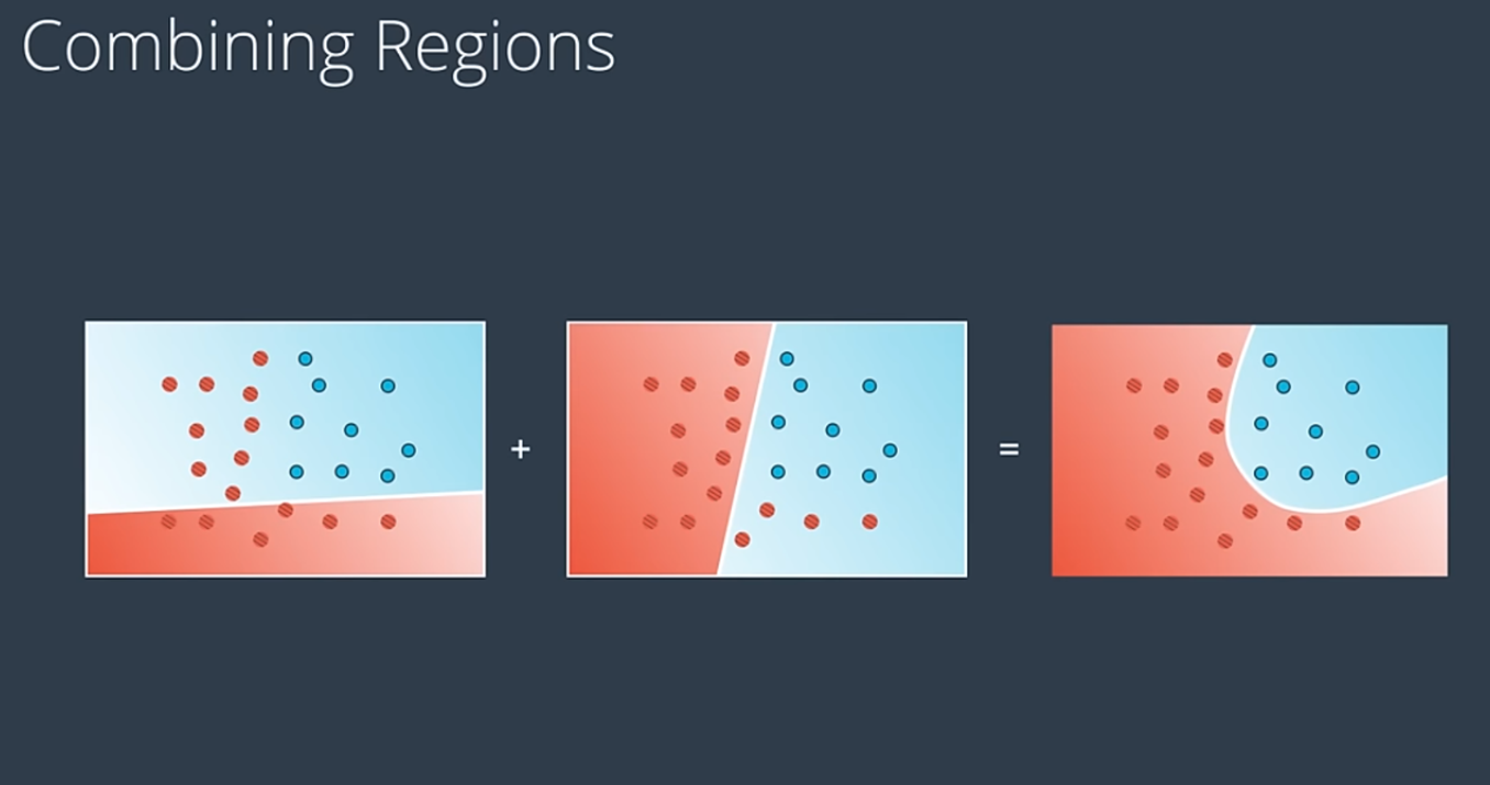
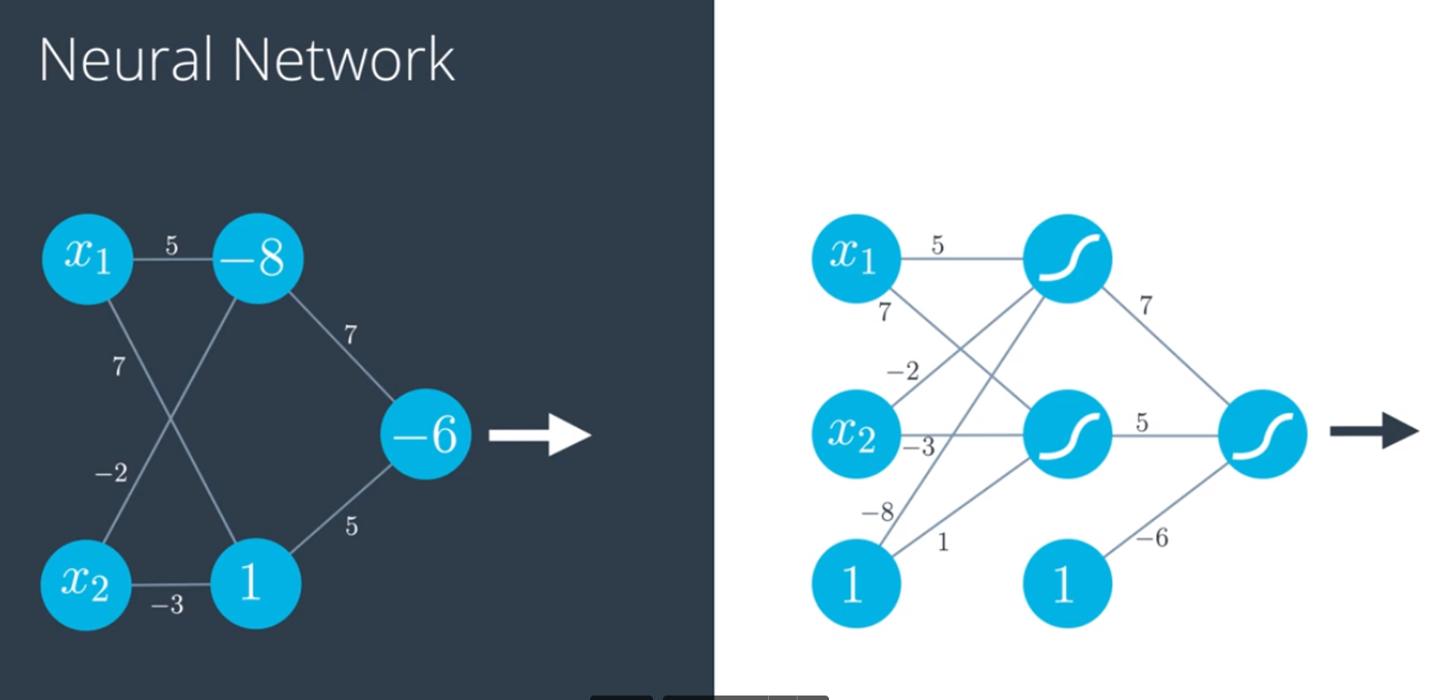
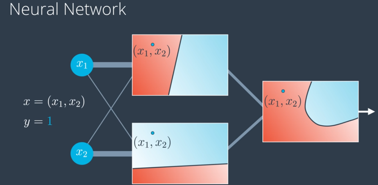
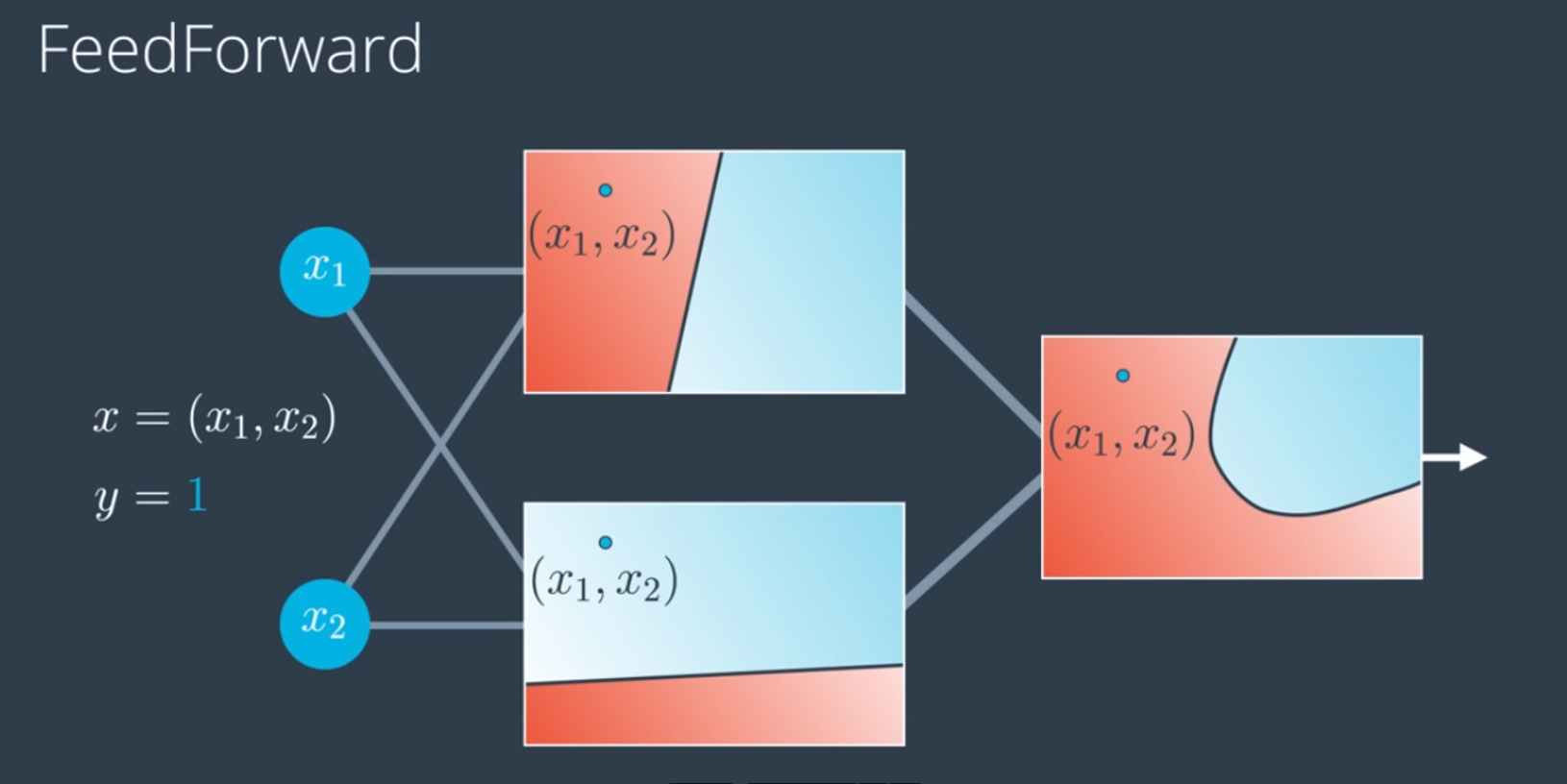
We will combine two linear models to get our non-linear model. Essentially the steps to do this are:

• Calculate the probability for each model
• Apply weights to the probabilities
• Add the weighted probabilities
• Apply the sigmoid function to the result

#Multiple layers

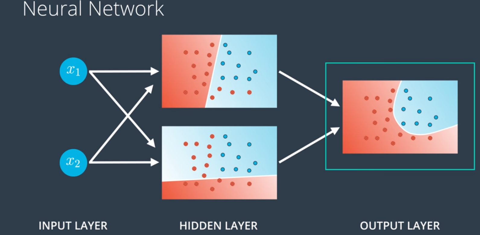
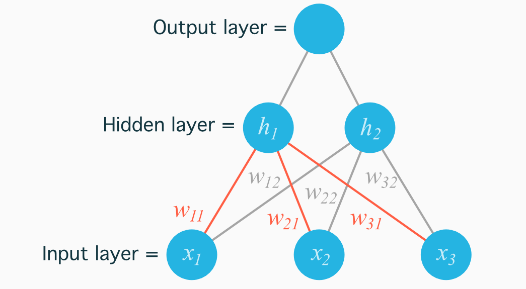
Neural networks have a certain special architecture with layers:

• The first layer is called the input layer, which contains the inputs.
• The next layer is called the hidden layer, which is the set of linear models created with the input layer.
• The final layer is called the output layer, which is where the linear models get combined to obtain a nonlinear model.

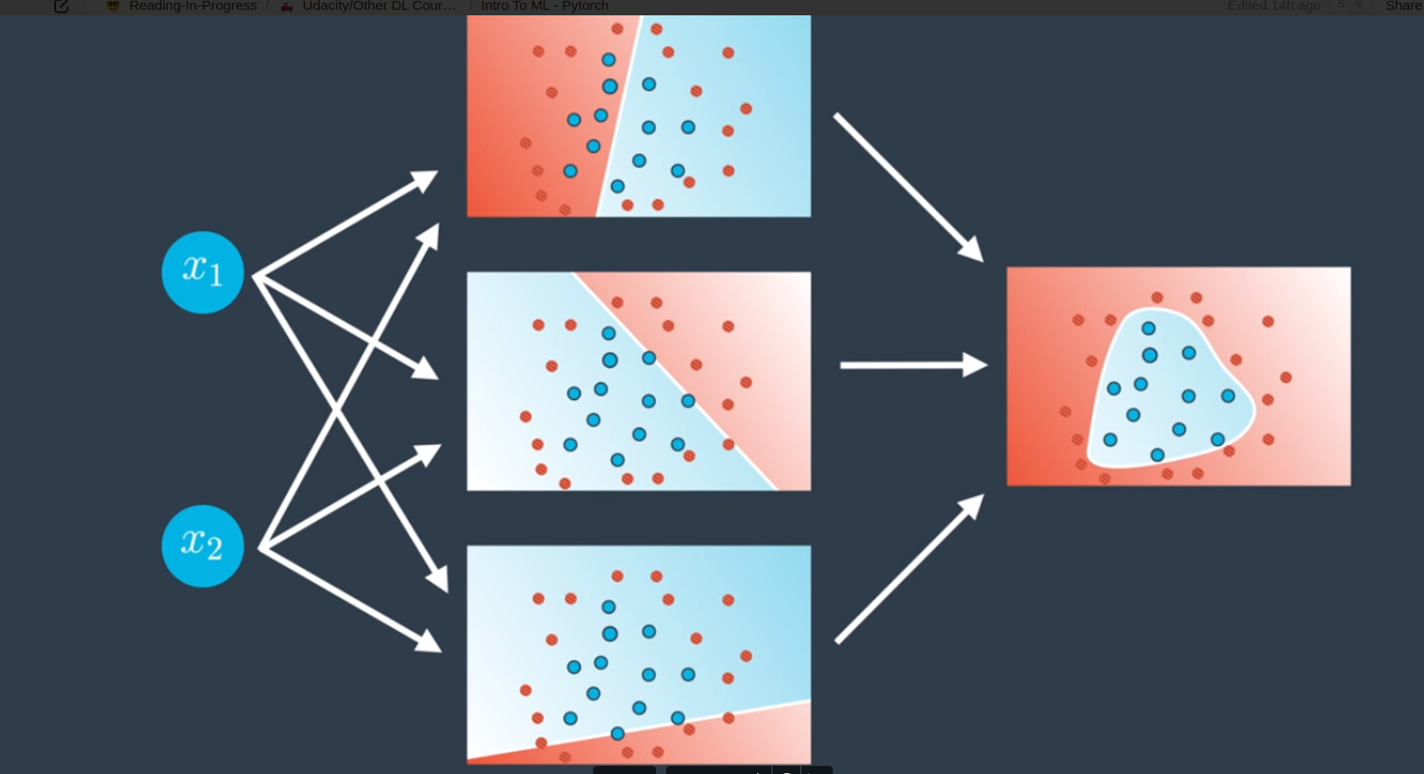
Neural networks can have different architectures, with varying numbers of nodes and layers:

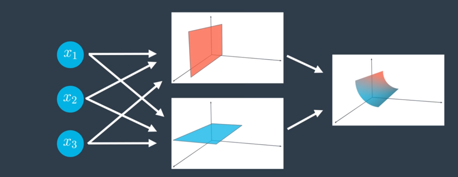
• Input nodes. In general, if we have n nodes in the input layer, then we are modeling data in n-dimensional space (e.g., 3 nodes in the input layer means we are modeling data in 3-dimensional space).
• Output nodes. If there are more nodes in the output layer, this simply means we have more outputs—for example, we may have a multiclass classification model.
• Layers. If there are more layers then we have a deep neural network. Our linear models combine to create nonlinear models, which then combine to create even more nonlinear models!

#Feedforward Intuition

Training a neural network essentially means determining what parameters they should have on the edges in order to model our data well. So in order to learn how to train them, we need to look carefully at how they process the input to obtain an output.

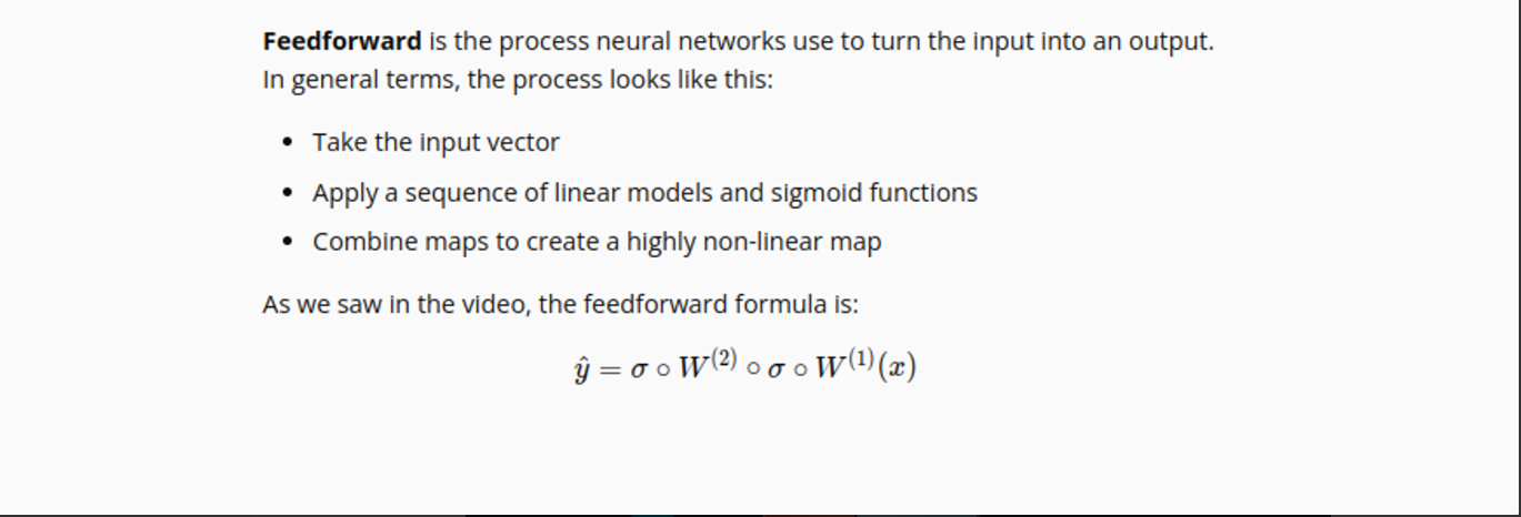
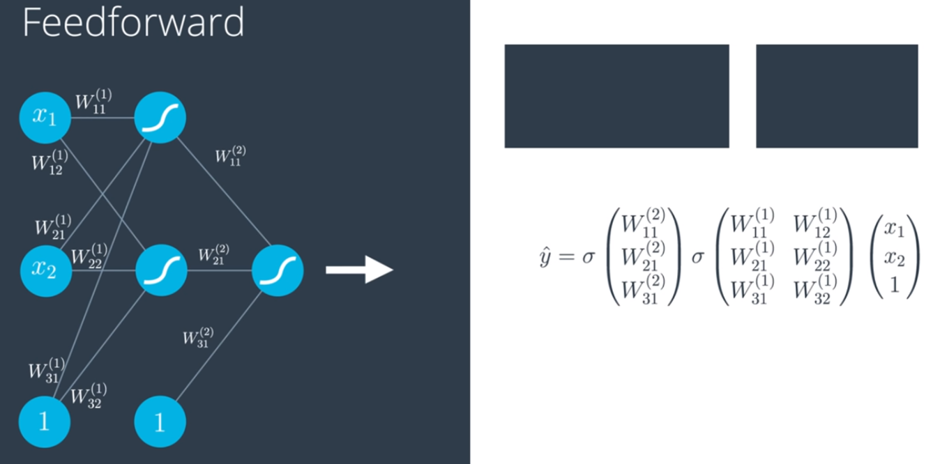
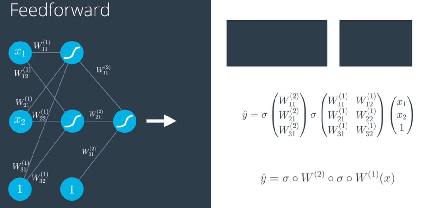
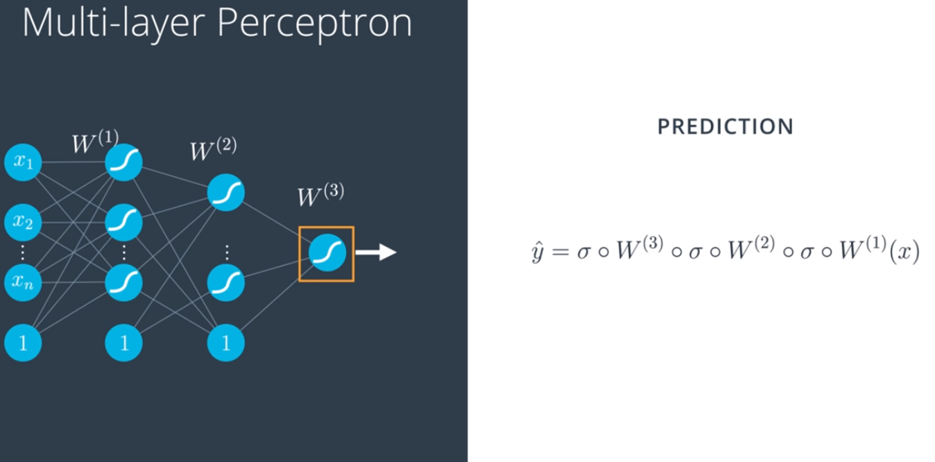
Just as before, neural networks will produce an error function, which at the end, is what we’ll be minimizing. For a multilayer perceptron, as we saw, our prediction is simply a combination of matrix multiplications and sigmoid functions. But the error function can be the exact same formula, aside from the fact that 𝑦^ is a bit more complicated.

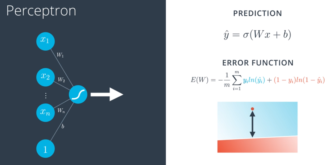
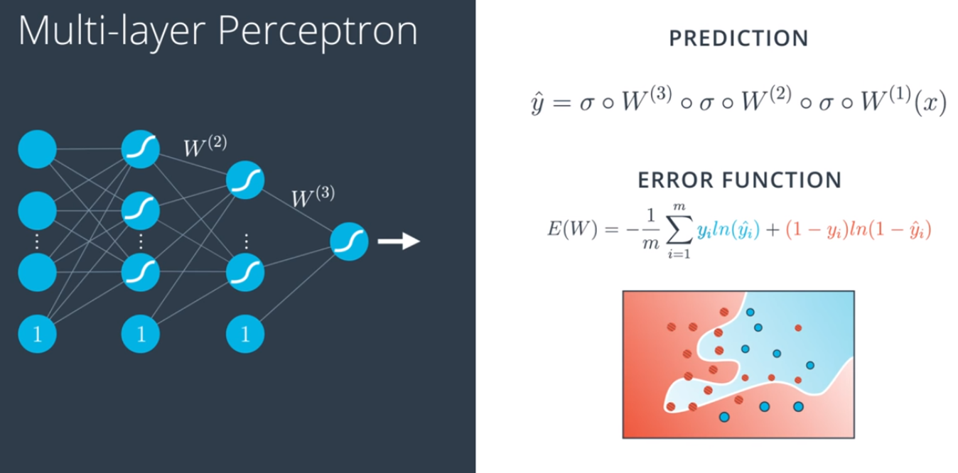
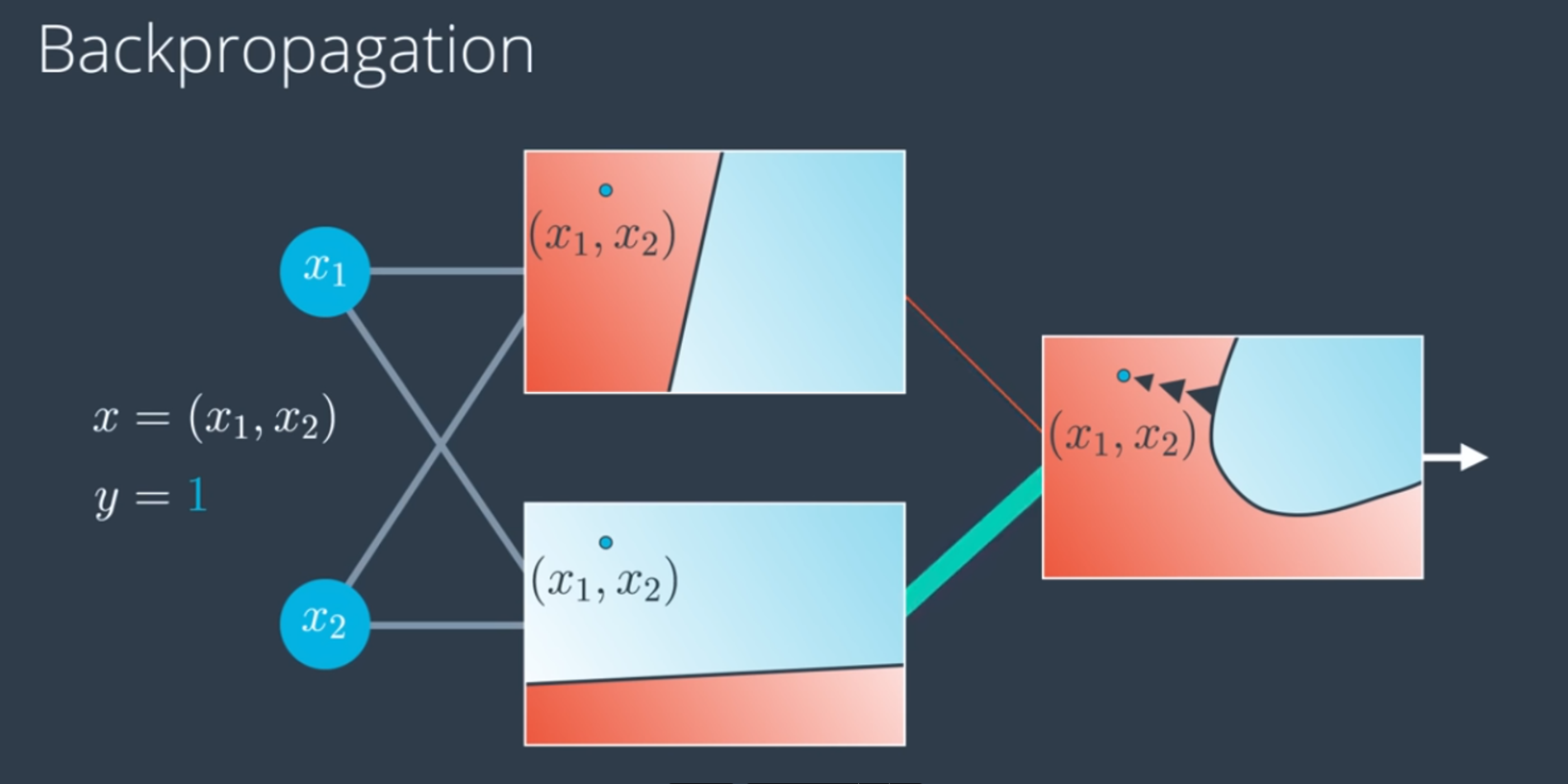
#Backpropagation Intution

In a nutshell, backpropagation will consist of:

• Doing a feedforward operation.
• Comparing the output of the model with the desired output.
• Calculating the error.
• Running the feedforward operation backwards (backpropagation) to spread the error to each of the weights.
• Use this to update the weights, and get a better model.
• Continue this until we have a model that is good.

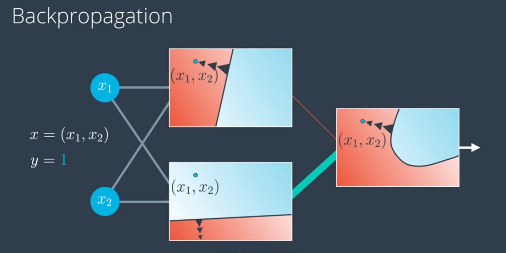
I refrain from going deep on derivatives in this post as it is covered in the above linked post related to Calculus.

#Hint

The following hint goes long way in debugging advanced Neural Network architectures

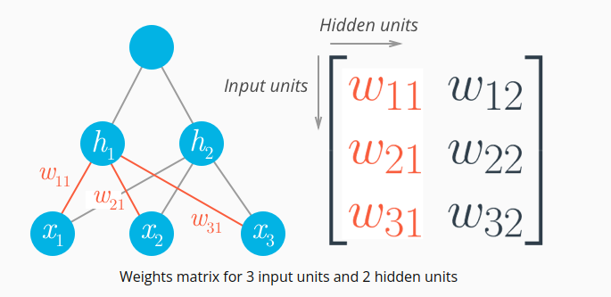
With single perceptron regression architectures, we are able to write the weights as an array, indexed as 𝑤𝑖. With multiple perceptron architecture, the weights need to be stored in a matrix, indexed as 𝑤𝑖𝑗

Each row in the matrix will correspond to the weights leading out of a single input unit, and each column will correspond to the weights leading in to a single hidden unit. For our three input units and two hidden units, the weights matrix looks like following

#Training Neural Network Best Practices

I like to highlight few of the best practices. Unless it is advanced architectures based on Recurrent Neural Architectures, Pytorch Lightning has lot of features for effective training.

1) Finding the right model which can generalize well for unseen data is crucial. Dividing the datasets into necessary splits and testing for generalization is important.

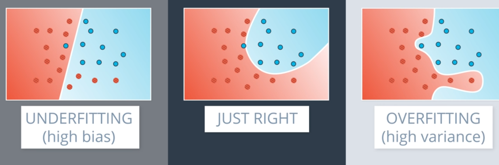
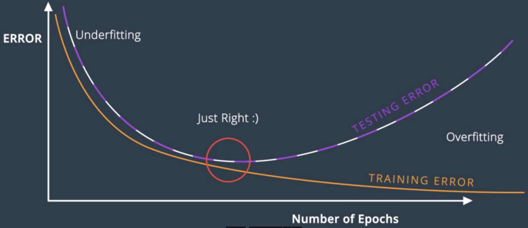
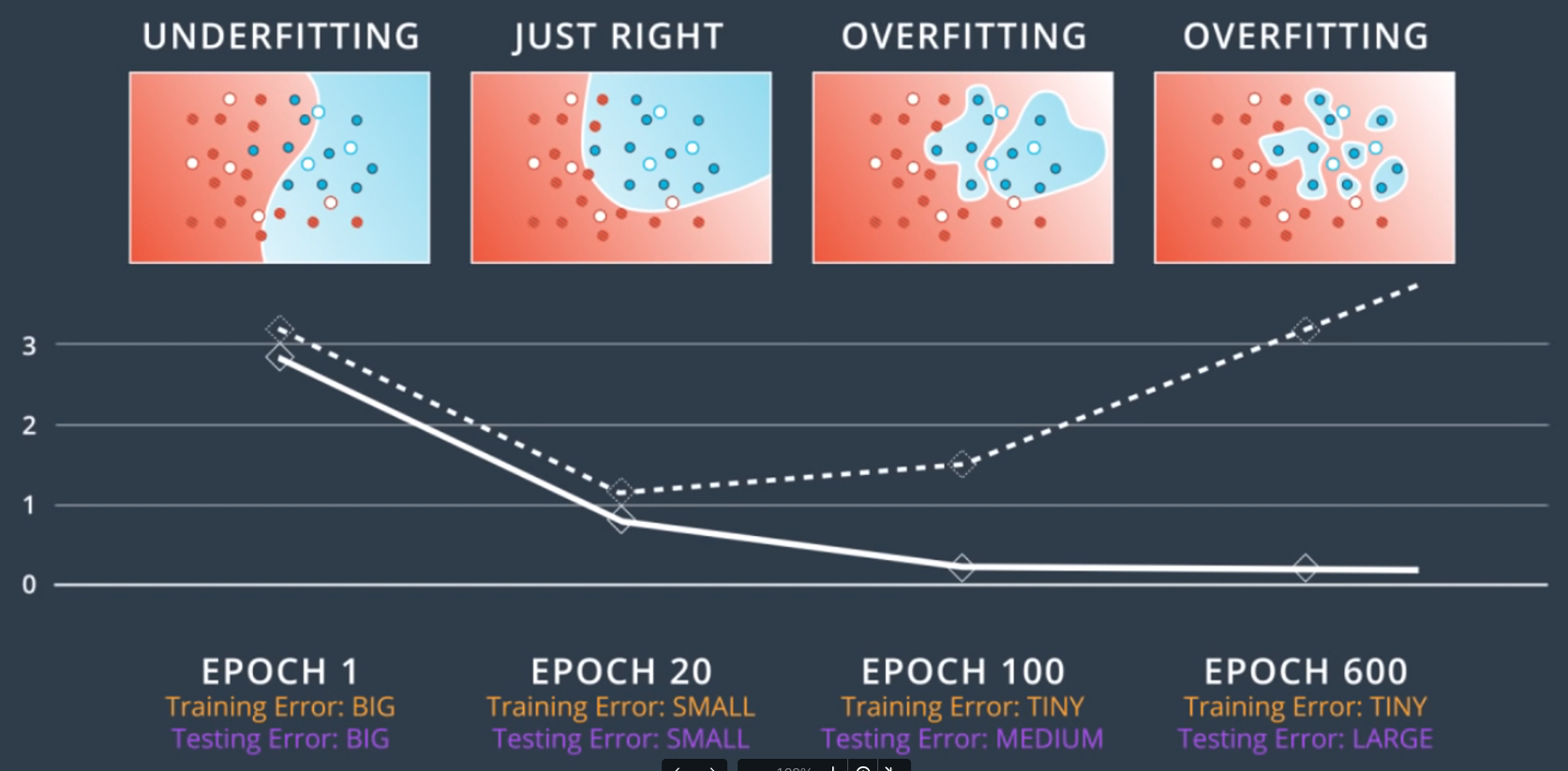
2) Early Stopping When training our neural network, we start with random weights in the first epoch and then change these weights as we go through additional epochs. Initially, we expect these changes to improve our model as the neural network fits the training data more closely. But after some time, further changes will start to result in overfitting.

We can monitor this by measuring both the training error and the testing error. As we train the network, the training error will go down—but at some point, the testing error will start to increase. This indicates overfitting and is a signal that we should stop training the network prior to that point. We can see this relationship in a model complexity graph

3) Regularization - L1 or L2, penalizing large weights and avoid overfitting.

#L1 vs L2 Regularization

The first approach (using absolute values) is called L1 regularization, while the second (using squares) is called L2 regularization. Here are some general guidelines for deciding between the two:

L1 Regularization

• L1 tends to result in sparse vectors. That means small weights will tend to go to zero.
• If we want to reduce the number of weights and end up with a small set, we can use L1.
• L1 is also good for feature selection. Sometimes we have a problem with hundreds of features, and L1 regularization will help us select which ones are important, turning the rest into zeroes.

L2 Regularization

• L2 tends not to favor sparse vectors since it tries to maintain all the weights homogeneously small.
• L2 gives better results for training models so it’s the one we’ll use the most.

4) Dropout - When training a neural network, sometimes one part of the network has very large weights and it ends up dominating the training, while another part of the network doesn’t really play much of a role (so it doesn’t get trained).

To solve this, we can use a method called dropout in which we turn part of the network off and let the rest of the network train:

• We go through the epochs and randomly turn off some of the nodes. This forces the other nodes to pick up the slack and take a larger part in the training.
• To drop nodes, we give the algorithm a parameter that indicates the probability that each node will get dropped during each epoch. For example, if we set this parameter to 0.2, this means that during each epoch, each node has a 20% probability of being turned off.
• Note that some nodes may get turned off more than others and some may never get turned off. This is OK since we’re doing it over and over; on average, each node will get approximately the same treatment.

5) Local Minima and Random Restart - Gradient descent looks at the direction where it can most decrease the error and then it takes a step in that direction. However, if there are multiple low points in the solution space, gradient descent may end up leading us to local minima—solutions where the error is at the lowest point in the local area, but not the lowest point overall.

One way to solve our problem is to use random restart. We start (and restart) from a few different random places and do gradient descend from all of them. This increases the probability that we’ll get to the global minimum, or at least a pretty good local minimum.

6) Batch vs Stochastic Gradient Descent

#Batch Gradient Descent

First, let’s review our batch gradient descent algorithm:

• In order to decrease error, we take a bunch of steps following the negative of the gradient, which is the error function.
• Each step is called an epoch.
• In each epoch, we take our input (all of our data) and run it through the entire neural network.
• Then we find our predictions and calculate the error (how far the predictions are from the actual labels).
• Finally, we back-propagate this error in order to update the weights in the neural network. This will give us a better boundary for predicting our data.
• If we have a large number of data points then this process will involve huge matrix computations, which would use a lot of memory.

#Stochastic Gradient Descent

To expedite this, we can use only some of our data at each step. If the data is well-distributed then a subset of the data can give us enough information about the gradient.

This is the idea behind stochastic gradient descent. We take small subsets of the data and run them through the neural network, calculating the gradient of the error function based on these points and moving one step in that direction.

We still want to use all our data, so what we do is the following:

• Split the data into several batches.
• Take the points in the first batch and run them through the neural network.
• Calculate the error and its gradient.
• Back-propagate to update the weights (which will define a better boundary region).
• Repeat the above steps for the rest of the batches.

Notice that with this approach we take multiple steps, whereas with batch gradient descent we take only one step with all the data. Each step may be less accurate, but, in practice, it’s much better to take a bunch of slightly inaccurate steps than to take only one good one.

7) Learning Rate Decay

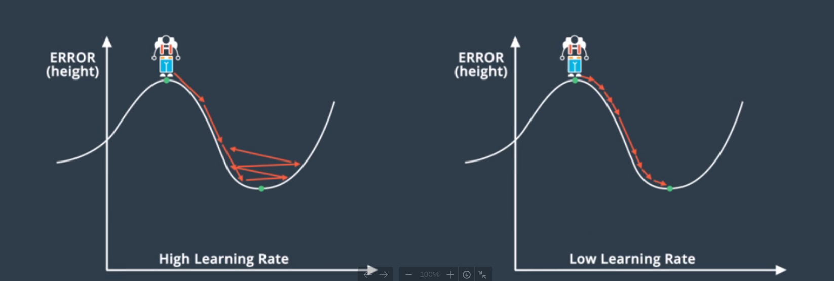
If the learning rate is large:

• This means the algorithm is taking large steps, which can make it faster.
• However, the large steps may cause it to miss (overshoot) the minimum.

If the learning learning rate is small:

• This means the algorithm is taking small steps, which can make it slower.
• However, it will make steady progress and have a better chance of arriving at the local minimum.

If your model is not working, a good general rule of thumb is to try decreasing the learning rate. The best learning rates are those that decrease as the algorithm is getting closer to a solution.

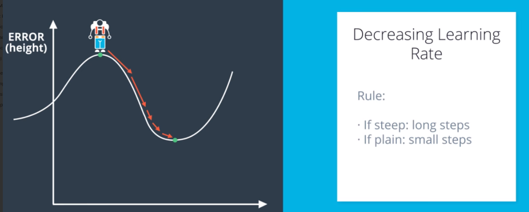
Frameworks like Pytorch Lightining has learning rate schedulers which helps with learning rate decay.

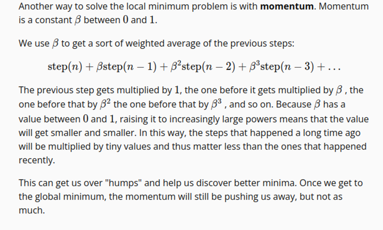
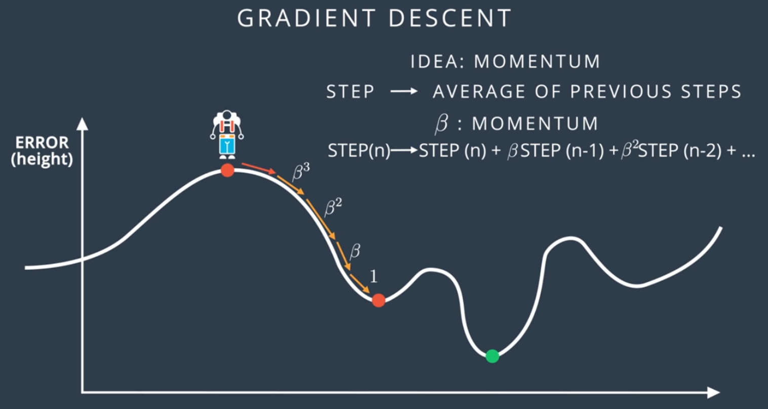
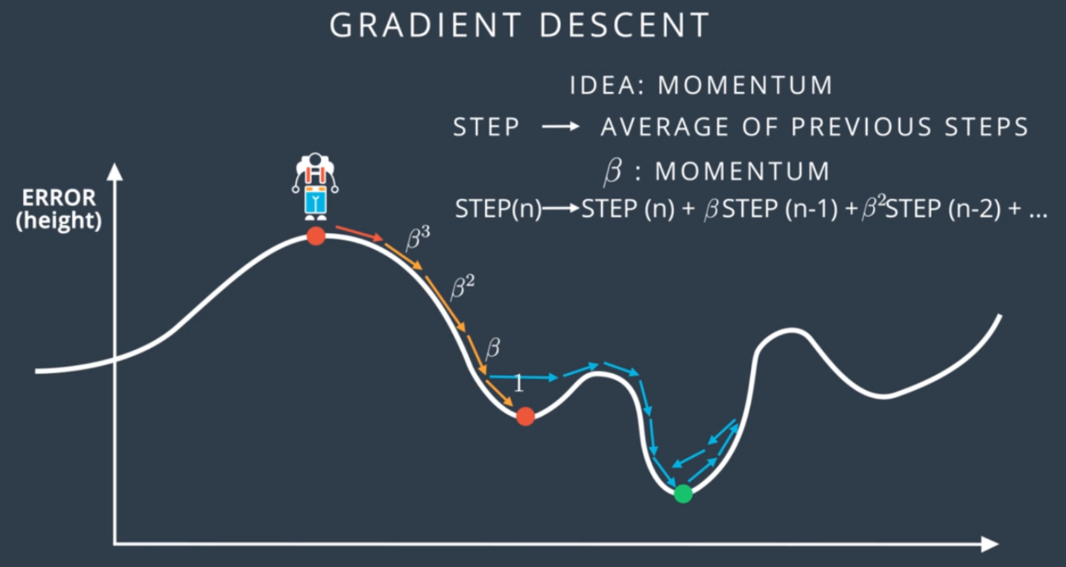
8) Momentum

#Points to remember

Cross entropy and maximum likelihood are closely related concepts in machine learning.

Maximum Likelihood Estimation (MLE):

• A statistical method to estimate the parameters of a probability distribution that best describes a given dataset.
• It aims to find the values of the parameters that maximize the likelihood function, which represents the probability of observing the actual data points given those parameters.
• Used in various machine learning tasks, including training models.

Cross Entropy:

• A measure of the difference between two probability distributions.
• In machine learning, it’s often used as a loss function during model training.
• The goal is to minimize the cross entropy between the predicted probability distribution (from the model) and the true probability distribution (representing the desired output).

The Connection:

• There’s a strong link between MLE and cross entropy. In many cases, minimizing the cross entropy loss function is equivalent to maximizing the likelihood function.
• This happens because the negative log-likelihood (which emphasizes low probabilities for incorrect predictions) is mathematically proportional to the cross entropy.

Here’s an analogy:

• Imagine you’re trying to find the best fitting hat for your head.
• MLE is like trying different hat sizes to see which one fits the most snugly (maximizing the likelihood of a good fit).
• Cross entropy is like measuring the gap between your head and the hat (a smaller gap indicates a better fit).

Key Points:

• Minimizing cross entropy often leads to maximizing likelihood (but it’s not always a perfect equivalence).
• They both serve the purpose of guiding the training process towards a model that performs well.
• Cross entropy is a more general concept used in various applications, while MLE is specifically about estimating probability distribution parameters.

In conclusion, while they are not identical, cross entropy and maximum likelihood are intertwined concepts. Minimizing cross entropy during training often leads to finding the model parameters that maximize the likelihood of the model making accurate predictions.

#References and Image credits

• Coursera, Deeplearning.ai - ML Specialization by Prof. Andrew Ng
• Udacity (image credits) and great teacher, again Lois Serrano.
• Yes, you should understand Backprod
• Why momementum works