The Two Pillars of Modern Generative AI: Contrastive Learning & Flow Matching
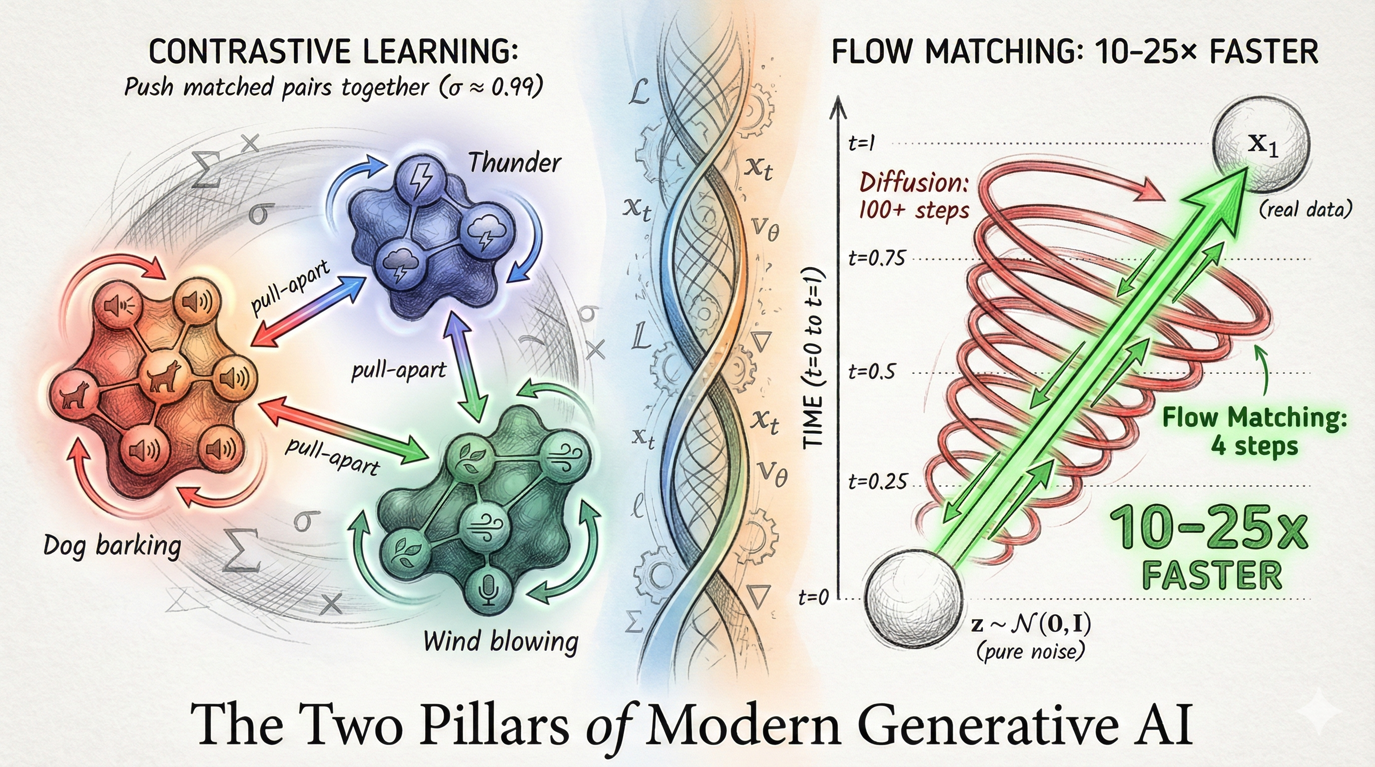
The Two Pillars of Modern Generative AI: Contrastive Learning & Flow Matching
All modern generative AI, from Image DiT to audio-video synthesis, uses two core concepts: contrastive learning for alignment and flow matching for efficient generation.
Table of Contents
- Introduction
- The Two Pillars: Contrastive Learning and Flow Matching
- Model 1: Image DiT
- Model 2: VACE
- Model 3: LTX-2
- Model 4: SAM Audio
- PE-AV: The Alignment Foundation
- Unified Insight: Contrastive + Flow Matching
- Practical Implications and Future Directions
- Conclusion
- References
- Appendix: Contrastive Learning in PE-AV
Diffusion Transformers in Latent Space: From Images to Audio-Visual Generation and Separation
Introduction
In an earlier post on latent space and latent encoding, we established a simple but powerful idea: instead of working directly with high-dimensional data (pixels, waveforms), we encode data into a learned latent space where a Diffusion Transformer (DiT) learns a generative trajectory. This post extends that story to four concrete, modern instantiations spanning images, video, joint audio-video, and audio separation: Stable Diffusion-style image DiTs, VACE (all-in-one video creation), LTX-2 (joint audio-video generation), and SAM Audio (multimodal audio separation).
Most importantly, we now include PE-AV (Perception Encoder AudioVisual), a foundational model that shows how to scale contrastive learning across audio, video, and text modalities, unlocking the alignment that powers SAM Audio’s multimodal conditioning and setting the stage for the next generation of unified encoders.
The diagram below captures all four models (plus PE-AV as the alignment backbone) under a unified lens:
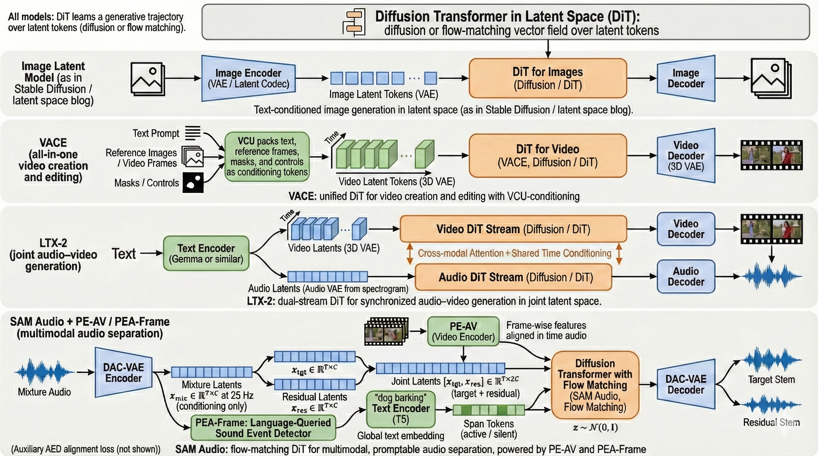
Each row represents a different task, but they all share the same generative backbone: a Transformer that learns a vector field in a compressed latent space.
🔑 What does this mean?
- Compressed latent space: Instead of working with raw pixels or waveforms, data is first encoded into a compact representation (covered in depth in our latent space blog).
- Vector field: At every point in this latent space, the model learns a velocity (direction + magnitude) that tells it how to move from noise toward real data. Think of it like a wind map: at every location, there’s an arrow pointing toward the destination.
- Transformer: The neural network architecture (with attention mechanisms) that predicts these velocities, conditioned on text, images, or other inputs.
By understanding one model, you understand the pattern that powers all of them.
The Two Pillars: Contrastive Learning and Flow Matching
All four models, and PE-AV at their foundation, rely on two mathematical concepts that appear across nearly every modern generative and multimodal model. Understanding these deeply is the key to understanding the entire landscape.
Pillar 1: Contrastive Learning (Appears in ALL 4 Models)
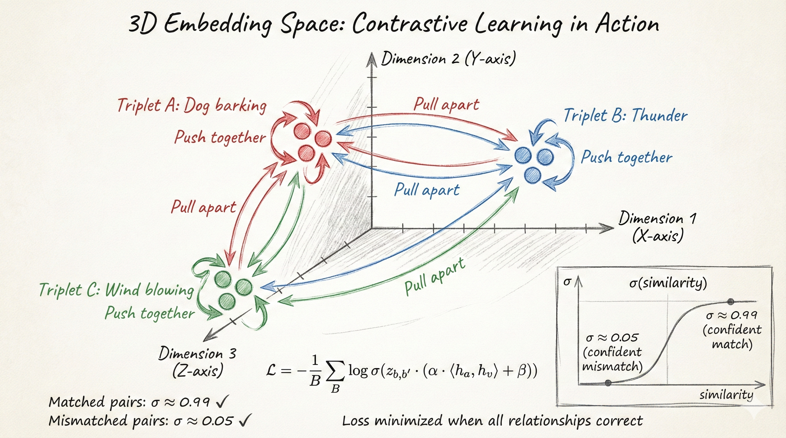
The Intuition: Imagine you have a million audio clips, video frames, and text captions. Your job is to arrange them in a high-dimensional space so that matching triplets (a sound, its video, and a text description) huddle together, while mismatches are pushed far apart. That’s contrastive learning.
🌟 Why It’s Everywhere
| Model | How It Uses Contrastive Learning |
|---|---|
| 🧠 PE-AV | 8 different contrastive loss pairs (audio-text, video-text, audio-video, etc.) simultaneously |
| 🎧 SAM Audio | Frame-level contrastive objectives (PEA-Frame) to align each audio frame with event descriptions |
| 🎬 LTX-2 | Cross-modal attention requires shared embedding spaces learned via contrastive objectives |
| 🖼️ Image DiT | Aligns text embeddings with image latents through contrastive learning |
📐 The Math: Sigmoid Contrastive Loss
Goal: Push matching pairs together, pull mismatched pairs apart in embedding space.
📥 Inputs
| Symbol | Meaning |
|---|---|
| h_a^b | Audio embedding for sample b (dimension C_h) |
| h_v^b | Video embedding for sample b (dimension C_h) |
| B | Batch size |
| α, β | Temperature and bias (learnable) |
| σ | Sigmoid function |
| z_bb′ | Indicator: +1 if matched (b=b′), -1 if mismatched |
🔢 The Loss Function
L(h_a, h_v) = -1/B * Σ_b Σ_b′ log σ( z_bb′ · (α · ⟨h_a^b, h_v^b′⟩ + β) )🪜 Step-by-Step Breakdown
| Step | Operation | What It Does |
|---|---|---|
| 1️⃣ | Similarity: s = ⟨h_a^b, h_v^b′⟩ | Dot product of normalized embeddings |
| 2️⃣ | Scale: s′ = α · s + β | Apply learned temperature & bias |
| 3️⃣ | Sigmoid: p = σ(s’) = 1/(1+e^(-s’)) | Convert to probability |
| 4️⃣ | Loss: -log(p) or -log(1-p) | Penalize wrong predictions |
| 5️⃣ | Average | Mean over all pairs in batch |
💡 The Intuition
| Scenario | What Happens | Network Learns To… |
|---|---|---|
| b = b′ (matched pair) | Maximize log σ(…) → push σ → 1 | Be confident they match ✅ |
| b ≠ b′ (mismatched) | Maximize -log(1-σ(…)) → push σ → 0 | Be confident they don’t match ❌ |
🧮 Numerical Example (Batch Size = 2)
Setup: Let’s walk through a concrete example with 2 audio-video pairs.
📋 Given Data
| Parameter | Value |
|---|---|
| Batch size | 2 samples |
| Embedding dimension | 3 |
| Temperature (α) | 10 |
| Bias (β) | 0 |
Embeddings (normalized):
| Sample | Audio Embedding | Video Embedding | Relationship |
|---|---|---|---|
| 1 | [0.8, 0.0, 0.6] | [0.7, 0.1, 0.7] | ✅ Matched |
| 2 | [-0.5, 0.8, 0.3] | [-0.4, 0.9, 0.1] | ✅ Matched |
1️⃣ Compute All Similarities
| Pair | Calculation | Result | Status |
|---|---|---|---|
| s₁,₁ | 0.8×0.7 + 0×0.1 + 0.6×0.7 | 0.98 | ✅ Matched (GOOD!) |
| s₁,₂ | 0.8×(-0.4) + 0×0.9 + 0.6×0.1 | -0.26 | ❌ Mismatch |
| s₂,₁ | (-0.5)×0.7 + 0.8×0.1 + 0.3×0.7 | -0.06 | ❌ Mismatch |
| s₂,₂ | (-0.5)×(-0.4) + 0.8×0.9 + 0.3×0.1 | 0.95 | ✅ Matched (GOOD!) |
2️⃣ Scale by Temperature (α=10)
| Pair | Calculation | Scaled Value |
|---|---|---|
| s′₁,₁ | 10 × 0.98 | 9.8 |
| s′₁,₂ | 10 × (-0.26) | -2.6 |
| s′₂,₁ | 10 × (-0.06) | -0.6 |
| s′₂,₂ | 10 × 0.95 | 9.5 |
3️⃣ Apply Sigmoid
| Pair | σ(s′) | Interpretation |
|---|---|---|
| σ(9.8) | 0.9994 | 🎯 Very confident: matched! |
| σ(-2.6) | 0.0690 | ✅ Confident mismatch |
| σ(-0.6) | 0.3543 | 🤔 Uncertain (could be better) |
| σ(9.5) | 0.9993 | 🎯 Very confident: matched! |
4️⃣ Compute Loss
L = -1/2 × [log(0.9994) + log(1-0.0690) + log(1-0.3543) + log(0.9993)]
  = -1/2 × [(-0.0006) + (-0.072) + (-0.438) + (-0.0007)]
  = -1/2 × (-0.512)
= 0.256💡 Takeaway
| Metric | Value | Meaning |
|---|---|---|
| Our loss | 0.256 | Low = good! |
| Random embeddings | ~0.69 | Maximum entropy |
| Matched pair confidence | ~99.9% | Excellent! |
| Mismatch confidence | 7-35% | Network knows they don’t match |
Visual: Contrastive Learning in Action
Pillar 2: Flow Matching (Emerging Standard for Latent Diffusion)
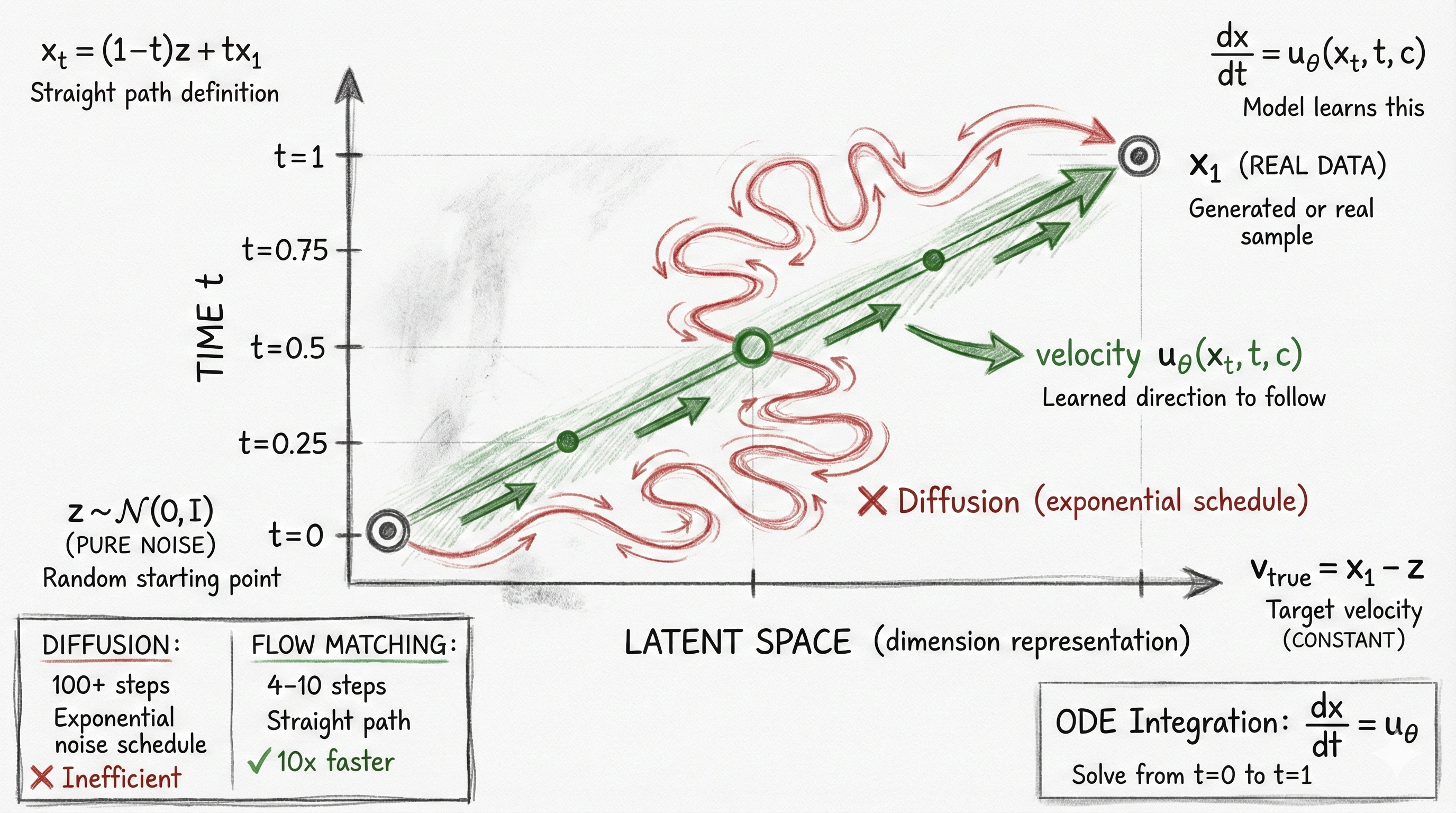
The Intuition: Instead of the multi-step noising process of traditional diffusion, imagine a straight line from noise (a random point) to data (a real datapoint). You learn to follow this line in the right direction at each point along the path. This is much faster and more elegant.
🌟 Why It Matters
| Model | Flow Matching Usage |
|---|---|
| 🎧 SAM Audio | Primary training objective (faster, more stable) |
| 🎬 LTX-2 | Offers both diffusion & flow matching (FM increasingly preferred) |
| 🔮 Future Models | Many new models adopting flow matching over diffusion |
📐 The Math: Flow Matching (Straight Path from Noise to Data)
Goal: Learn a velocity field that transports random noise to real data along a straight path.
📥 Setup
| Symbol | Meaning |
|---|---|
| z ~ N(0, I) | Random noise (starting point) |
| x₁ | Real data (ending point) |
| t ∈ [0, 1] | Time along the path |
🛤️ The Straight Path
x_t = (1 - t) · z + t · x₁| Time | Position | Meaning |
|---|---|---|
| t = 0 | x₀ = z | 🎲 Pure noise |
| t = 1 | x₁ = x₁ | 🎯 Real data |
⚡ True Velocity (Ground Truth)
dx/dt = d/dt[(1-t) · z + t · x₁] = x₁ - z🔑 Key insight: This is a CONSTANT vector field! The velocity doesn’t change along the path.
🎯 Training Objective
L_FM = E[ || u_θ(x_t, t, c) - (x₁ - z) ||² ]| Term | Meaning |
|---|---|
| u_θ | Neural network (velocity predictor) |
| x_t | Current position at time t |
| c | Conditioning (text, video, etc.) |
| (x₁ - z) | Target velocity to learn |
🚀 Inference (4 Simple Steps)
| Step | Action |
|---|---|
| 1️⃣ | Sample z ~ N(0, I) |
| 2️⃣ | Solve ODE: dx/dt = u_θ(x, t, c) from t=0 → t=1 |
| 3️⃣ | Result x₁ lies on learned data manifold |
| 4️⃣ | Decode: data = D(x₁) |
⚡ Why Flow Matching is Faster
| Method | Steps Needed | Path Shape |
|---|---|---|
| Diffusion | 50-1000 | Exponential noise schedules 📈 |
| Flow Matching | 10-20 | Straight line → fast ODE solvers ➡️ |
Result: Same (or better) quality with 5-50x speedup! 🎉
🧮 Numerical Example: Learning a Straight Path (1D Case)
The Setup: Imagine teaching a neural network to travel from point A to point B in a straight line. We’ll use a simple 1D example to build intuition.
Given: | Symbol | Value | Meaning | |--------|-------|---------| | z | -3.0 | Starting point (random noise) | | x₁ | +5.0 | Destination (real data) | | v_true | 8.0 | Velocity needed: 5.0 - (-3.0) = 8.0 |
📍 The Journey: Interpolating from Noise to Data
The magic formula: x_t = (1-t) · z + t · x₁
Think of t as “how far along the journey” (0% → 100%):
| Time (t) | Position (x_t) | Where Are We? |
|---|---|---|
| 0.00 | -3.0 | 🚀 Start: Pure noise |
| 0.05 | -2.6 | Just departed… |
| 0.10 | -2.2 | Getting warmer |
| 0.20 | -1.4 | Leaving the noise behind |
| 0.50 | 1.0 | 🎯 Halfway there! |
| 0.80 | 3.4 | Almost home |
| 1.00 | 5.0 | ✅ Arrived: Real data! |
🎓 What the Network Learns
At every point along this journey, we teach the network: “No matter where you are, the velocity is always 8.0”
| Training Input | Target Output |
|---|---|
| (x_t = -3.0, t = 0.00) | v = 8.0 |
| (x_t = -2.6, t = 0.05) | v = 8.0 |
| (x_t = -2.2, t = 0.10) | v = 8.0 |
| … | … |
| (x_t = 3.4, t = 0.80) | v = 8.0 |
| (x_t = 5.0, t = 1.00) | v = 8.0 |
Key insight: The velocity is constant because we’re learning a straight-line path. The network learns: “always move at speed 8.0 toward the destination.”
Inference with 4 Steps (Euler Method):
Initial: x = z = -3.0, t = 0
dt = 1 / 4 = 0.25

Step 1 (t=0.00→0.25):
  v_pred = u_θ(-3.0, 0.00, c) ≈ 8.0  (trained to predict this)
  x_new = x + v_pred * dt = -3.0 + 8.0*0.25 = -1.0

Step 2 (t=0.25→0.50):
  v_pred = u_θ(-1.0, 0.25, c) ≈ 8.0
  x_new = -1.0 + 8.0*0.25 = 1.0

Step 3 (t=0.50→0.75):
  v_pred = u_θ(1.0, 0.50, c) ≈ 8.0
  x_new = 1.0 + 8.0*0.25 = 3.0

Step 4 (t=0.75→1.00):
  v_pred = u_θ(3.0, 0.75, c) ≈ 8.0
  x_new = 3.0 + 8.0*0.25 = 5.0  ✓ (converged to x_1)
Result: In just 4 steps, we went from -3.0 to 5.0 exactly. With diffusion, this would require ~100+ steps with exponential noise schedules.
Visual: Flow Matching Trajectory
Model 1: Image DiT (Stable Diffusion Style)
Task: Text-to-image generation 🖼️
📦 Latent Space
| Component | Details |
|---|---|
| Encoder | Standard VAE (e.g., Stable Diffusion) |
| Shape | z ∈ ℝ^(H′ × W′ × C) |
| Compression | 512×512 image → 8×8 latent with 4 channels (~4000× smaller!) |
🎯 Conditioning Pipeline
📝 Text Prompt
     ↓
🧠 Pre-trained Text Encoder (CLIP)
     ↓
📤 Token Embeddings: c_text ∈ ℝ^(N × d)
     ↓
🔗 Cross-Attention in DiT blocks🎯 Objective
- Training: Predict noise (or score) at each step, conditioned on text
- Inference: Sample Gaussian noise → denoise iteratively → image!
💡 Why Latent Space Wins
| Pixel Space | Latent Space |
|---|---|
| 512 × 512 × 3 = 786K values | 8 × 8 × 4 = 256 values |
| Expensive to model | ⚡ Orders of magnitude cheaper |
| Includes perceptual noise | VAE filters out irrelevance |
Model 2: VACE (All-in-One Video Creation and Editing)
Task: Text and image-guided video generation and editing 🎬
📦 Latent Space
| Component | Details |
|---|---|
| Encoder | 3D Video VAE (space-time volumetric compression) |
| Shape | x ∈ ℝ^(T × H′ × W′ × C) |
| Example | 16-frame video → 16 × 16 × 16 × 16 latent tokens |
🎮 Conditioning (VCU: Video Condition Unit)
| Input Type | Purpose |
|---|---|
| 📝 Text prompt | Describe desired video or edits |
| 🖼️ Reference images/frames | Visual anchors or style guidance |
| 🎨 Masks/controls | Spatial regions to edit or preserve |
All packed into a unified conditioning token sequence → fed to DiT
🎯 Objective
- Diffusion-style: DiT learns to denoise (or flow-match) video latents conditioned on VCU
🚀 Why This Architecture Scales
- Single backbone handles both creation AND editing (just different conditioning)
- Spatial + temporal structure in latent helps Transformer reason about video coherence
Model 3: LTX-2 (Joint Audio-Video Generation)
Task: Synchronized text-to-audio-video generation 🎵🎬
📦 Latent Space (Dual Stream)
| Stream | Encoder | Shape | Scale |
|---|---|---|---|
| 🎬 Video | 3D Video VAE | x_v ∈ ℝ^(T_v × H′ × W′ × C_v) | ~14B params |
| 🎙️ Audio | Audio VAE (spectrogram) | x_a ∈ ℝ^(T_a × C_a) | ~5B params |
🔑 Key: Time stamps are aligned via resampling → audio and video latents stay synchronized!
🎮 Conditioning
📝 Text Prompt
     ↓
🧠 Text Encoder (Gemma or similar)
     ↓
   ┌───────────────────┬───────────────────┐
   ↓                   ↓
🎬 Video DiT          🎙️ Audio DiT
   ↓                   ↓
   └───── Cross-Modal Attention ─────┘
(shared time embeddings)🎯 Objective
L = L_video + L_audio (parallel diffusion/flow-matching losses)- Cross-modal attention terms to align semantics across modalities
💡 Why Dual-Stream + Cross-Modal?
| Challenge | Solution |
|---|---|
| Audio & video have different temporal scales | Separate streams = more efficient |
| Need synchronized generation | Shared time conditioning |
| Avoid single bottleneck | Cross-attention instead of fusion |
Model 4: SAM Audio (Multimodal Audio Separation)
Task: Text, visual, or temporal prompts → separate target sound from a mixture 🎧
📦 Latent Space
| Component | Shape | Purpose |
|---|---|---|
| Mixture | x_mix ∈ ℝ^(T × 128) | Input audio (conditioning only) |
| Target | x_tgt ∈ ℝ^(T × 128) | Sound to extract |
| Residual | x_res ∈ ℝ^(T × 128) | Everything else |
| Joint output | [x_tgt, x_res] ∈ ℝ^(T × 256) | What DiT generates from noise |
Encoder: DAC-VAE @ 25 Hz (lower frame rate = shorter sequences)
🔑 Why DAC-VAE?
| Feature | Benefit |
|---|---|
| Continuous Gaussian latents | Essential for flow matching (no discrete codes) |
| Low frame rate (25 Hz) | Short sequences while preserving audio fidelity |
| VAE prior N(0, I) | Aligns perfectly with flow-matching start distribution |
🎮 Conditioning: Three Modalities Combined
1️⃣ Text Prompt
📝 "dog barking", "woman speaking"
        ↓
   🧠 T5 Encoder
        ↓
   📤 c_text ∈ ℝ^(N_txt × 768)
        ↓
🔗 Cross-attention in DiT blocks2️⃣ Visual Prompt (PE-AV)
🖼️ User selects region in video frames
        ↓
   🧠 Perception Encoder (PE)
        ↓
   📤 Frame-level features c_vid(t)
        ↓
   ⏱️ Resample to 25 Hz
        ↓
➕ Concatenate with audio latents3️⃣ Span Prompt (PEA-Frame)
| Mode | How It Works |
|---|---|
| Manual | User specifies time ranges (t_start, t_end) |
| Automatic | PEA-Frame predicts frame-wise activity |
Automatic detection:
  ℓ_l = cos_sim(audio_frame, text_embedding)
       ↓
  Threshold → binary span tokens s_l ∈ {0, 1}
       ↓
Embed + concatenate with audio latents🎯 Training Objective: Two Losses Working Together
The Big Picture: Combine flow matching (the main generative signal) with semantic alignment (ensuring the model understands what sounds mean).
📊 The Combined Loss
L_total = L_FM + λ · L_aux| Component | What It Does |
|---|---|
| L_FM | Flow matching loss (main training signal) |
| L_aux | Auxiliary semantic alignment loss |
| λ | Balance weight between the two |
🌊 Flow Matching Loss (L_FM)
L_FM = E[ || u_θ([x_mix, c_vid, c_span], t, c_text) - (x₁ - z) ||² ]| Input | Meaning |
|---|---|
| x_mix | Mixed audio latent |
| c_vid | Video conditioning |
| c_span | Span (temporal) prompt |
| c_text | Text description |
| (x₁ - z) | Target velocity |
💡 This is the main training signal: learn to predict the velocity that takes noise → clean audio.
🔗 Auxiliary Semantic Alignment Loss (L_aux)
L_aux = E[ 1 - sim(a_l, a_tgt) ]| Term | Meaning |
|---|---|
| a_l | Learned audio representation |
| a_tgt | External AED model embedding |
| sim | Cosine similarity |
💡 This regularizer ensures the model’s internal representations align with a pretrained Audio Event Detection (AED) model.
🩹 Handling Missing Prompts
Not all training examples have all three modalities. Here’s how the model stays robust:
| Missing Modality | Fallback |
|---|---|
| 📝 Text | Empty string |
| 🎬 Video | All-zero feature sequence |
| ⏱️ Span | “null” tokens |
🎲 Training trick: Randomly drop each modality with probability (p_text, p_video, p_span) to encourage robustness at inference!
🧩 Why Joint Target + Residual?
| Benefit | Explanation |
|---|---|
| Coupled distribution | Extracting target forces a plausible residual (conservation of energy) |
| Simultaneous decoding | DAC-VAE decoder outputs both waveforms at once |
PE-AV: The Alignment Foundation for All Models
💡 Key Insight: SAM Audio, LTX-2, and even Image DiT all rely on aligned cross-modal embeddings. PE-AV (Perception Encoder AudioVisual) makes this alignment possible at scale.
🏗️ PE-AV Architecture
PE-AV uses a multi-tower design with 8 contrastive loss pairs:
📥 Input Streams
| Modality | Processing |
|---|---|
| 🎙️ Audio | Raw waveform → DAC-VAE (25 Hz tokens, 128 dim) |
| 🎬 Video | RGB frames (30 FPS) → PE-L frame encoder + temporal transformer (4 layers) |
| 📝 Text | Captions → ModernBERT (28 layers, 512 context length) |
🧠 Encoding Towers (all output 1024-dim embeddings)
| Tower | Architecture |
|---|---|
| Audio Transformer | 28 layers, 1.11B params (PEAV-L) |
| Video Transformer | 4 temporal layers on PE-L |
| Text Encoder | ModernBERT layer 22 |
| Audio-Video Fusion | 6 layers (concatenate + fuse) |
🔗 Contrastive Training: 8 Loss Pairs!
① Audio ↔ Audio Caption
② Audio ↔ Video
③ Audio ↔ Audio-Video Caption
④ Audio-Video ↔ Audio Caption
⑤ Audio-Video ↔ Audio-Video Caption
⑥ Video ↔ Audio Caption
⑦ Video ↔ Video Caption
⑧ Video ↔ Audio-Video Caption

(+ 2 more pairs during fine-tuning for joint text-conditioned retrieval)
🎯 Result: All 8 objectives train jointly → shared 1024-dimensional embedding space where audio, video, and text coexist!
🏆 PE-AV Results (vs. Previous SOTA)
| Benchmark | PE-AV | Previous Best | Improvement |
|---|---|---|---|
| AudioCaps text-to-audio | 45.8 | 35.4 | +10.4 |
| VGGSound classification | 47.1 | 36.0 | +11.1 |
| ActivityNet video-text retrieval | 66.5 | 60.4 | +6.1 |
| Speech retrieval (R@1) | 85.6 | ~0 | 🌟 First model to enable this! |
🧩 Unified Insight: Contrastive + Flow Matching as Universal Backbone
The four models above are not coincidentally similar. They arise naturally from combining two forces:
| Force | Role |
|---|---|
| 🔗 Contrastive Learning | Aligns modalities in embedding space (PE-AV proves this at scale) |
| 🌊 Flow Matching (or Diffusion) | Learns generative trajectories in that aligned latent space |
🛠️ The Modular, Composable System
| Component | Role | Appears in |
|---|---|---|
| 🔗 Contrastive Alignment | Learn shared embedding for multiple modalities | All 4 models + PE-AV |
| 🌊 Flow Matching | Fast, stable ODE integration from noise to data | SAM Audio (primary) |
| 🌀 Diffusion | Traditional multi-step reversal of noise process | Image DiT, VACE, LTX-2 |
| 🎯 Conditioning | Inject aligned embeddings as guidance | All 4 models |
🚀 Practical Implications and Future Directions
✨ Why This Matters Now
| Advantage | Impact |
|---|---|
| ⚡ Efficiency | Latent-space models are 10–100× faster to train and sample |
| 🌐 Flexibility | Same backbone adapts to images, video, audio, or mixtures |
| 📈 Scalability | DiT architectures scale cleanly; billion-parameter models are practical |
| 🔗 Alignment at Scale | PE-AV proves contrastive learning works in a single 1024-dim space |
🔮 What’s Coming
| Trend | Why It Matters |
|---|---|
| 🧩 Deeper multimodal fusion | LTX-2’s cross-modal attention hints at inseparable audio+video+text |
| 🎯 Sophisticated prompting | Frame-level, object-level, semantic-level conditioning becoming standard |
| 🌊 Flow matching dominance | Faster and more stable; expect it to replace diffusion |
| 🧠 Unified encoders everywhere | Pre-aligned multimodal embeddings will be baked in |
| ✏️ Beyond generation | Same recipe adapting to editing, inpainting, 3D generation |
🏁 Conclusion
From image generation to video creation to audio separation to multimodal alignment, the pattern is clear:
| Pillar | Role |
|---|---|
| 🔗 Contrastive Learning | Align embeddings across modalities |
| 🌊 Flow Matching (or Diffusion) | Learn generative trajectories in aligned space |
| 🧠 Transformers in Latent Space | Scale both to billions of parameters |
Understanding these three pillars deeply gives you intuition for virtually every modern generative and multimodal model. The unified diagram at the top of this post is not just a pretty picture. It’s a map of a conceptual territory that is increasingly central to AI.
📝 Three Ideas to Keep in Your Pocket
| Principle | Why |
|---|---|
| 1️⃣ Encode everything into latent space first | Orders of magnitude cheaper to model |
| 2️⃣ Use contrastive learning to align modalities | PE-AV shows this works at scale |
| 3️⃣ Use flow matching for fast, stable generation | Straight paths beat exponential schedules |
🌟 This is rapidly becoming the lingua franca of generative modeling.
It is rapidly becoming the lingua franca of generative modeling.
References
- Stable Diffusion / Latent Diffusion: https://arxiv.org/abs/2112.10752
- Diffusion Transformers (DiT): https://arxiv.org/abs/2212.09748
- VACE: https://arxiv.org/abs/2503.07598
- LTX-2: https://arxiv.org/abs/2601.03233
- SAM Audio: https://arxiv.org/abs/2501.08761
- PE-AV (Perception Encoder Audio-Visual): https://arxiv.org/abs/2411.12476
- PEA-Frame (frame-level audio-text alignment): Included in SAM Audio paper
Appendix: Contrastive Learning in PE-AV (8 Loss Pairs Explained)
PE-AV trains with 8 simultaneous contrastive objectives. Here’s why each pair matters:
PRETRAINING (8 pairs):
1. Audio → Audio Caption
   - Task: given audio embedding, retrieve correct audio caption
   - Why: semantic understanding of what's being heard

2. Audio ↔ Video
   - Task: given audio, find matching video (and vice versa)
   - Why: cross-modal alignment (essential for SAM Audio visual prompting)

3. Audio → Audio-Video Caption
   - Task: given audio, retrieve caption describing entire audio-visual scene
   - Why: connect individual modality to holistic scene understanding

4. Audio-Video ↔ Audio Caption
   - Task: given fused audio-video, retrieve audio-specific caption
   - Why: teaches fusion layer what audio contributes to scene

5. Audio-Video → Audio-Video Caption
   - Task: given fused audio-video embedding, retrieve full caption
   - Why: unified multimodal understanding

6. Video → Audio Caption
   - Task: given video frames, retrieve audio description
   - Why: visual understanding of audio content (e.g., "dog barking" from video of dog)

7. Video → Video Caption
   - Task: given video, retrieve visual caption
   - Why: standard video-text alignment (like ViT models)

8. Video → Audio-Video Caption
   - Task: given video, retrieve full audio-visual caption
   - Why: teaches video what audio adds to understanding

FINE-TUNING (2 additional pairs):
9. (Audio + Text) → Video
   - Task: retrieve video given both audio and text
   - Why: enables text-conditioned cross-modal retrieval

10. (Video + Text) → Audio
    - Task: retrieve audio given both video and text
    - Why: enables text-conditioned cross-modal retrieval
All 10 losses are computed simultaneously during training, creating a dense supervision signal that forces the embedding space to be rich enough for ANY combination of modalities.
This blog post is a companion to ”Latent Space and Latent Encoding”. For deeper dives into individual models, see the papers linked above. For implementation details, visit the PE-AV GitHub: https://github.com/facebookresearch/perception_models