#Understanding Latent Space and Latent Encoding: Theory, Math, and Context in DiT, VACE

#1. What Is Latent Space?

In machine learning, the term latent refers to something hidden or not directly observable. A latent space is a compressed, abstract vector space where high-dimensional data (like images) are mapped into a lower-dimensional representation that captures their essential features.

This transformation is done through a process called encoding, and the resulting latent vectors represent the most meaningful information about the original data.

Key Idea:
Latent space is a lower-dimensional, continuous, and structured representation of complex, high-dimensional data like images.

#Latent Space: Core Properties

• Lower Dimensionality: Reduces the number of variables needed to describe the data.
• Continuity: Small changes in latent space correspond to small, meaningful changes in output.
• Structure: Similar inputs cluster together; interpretable directions may exist (e.g., “add glasses”, “smile”).

---

#2. What Is Latent Encoding?

Latent encoding is the process of mapping input data (e.g., an image) into a latent vector—a point in the latent space. This is typically performed by a neural network called an encoder.

The reverse process—mapping from latent space back to the original data space—is handled by a decoder.

#Encoder-Decoder Framework

Input Data  →  Encoder  →  Latent Vector
                             ↓
                        Decoder
                             ↓
                        Reconstructed Data

#Why Use Latent Encoding?

• Efficiency: Reduces computational load by working with fewer dimensions.
• Abstraction: Focuses on semantic meaning rather than raw pixel values.
• Generative Power: Enables interpolation, editing, and synthesis of new data.

---

#3. Latent Encoding in DiT: The Diffusion Transformer Pipeline

In DiT (Diffusion Transformers), latent encoding plays a central role in how images are processed and generated.

#DiT Latent Encoding Workflow

Image (High-Dim)  
     ↓  
VAE Encoder → Latent Tensor (e.g., 32×32×4)  
     ↓  
Patchify → Sequence of Vectors  
     ↓  
Add Noise (Diffusion Step)  
     ↓  
DiT Transformer → Denoises in Latent Space  
     ↓  
VAE Decoder → Reconstructs Final Image

#Example Dimensions

- Input Image: $256 \times 256 \times 3 = 196,608$ values
- Encoded Latent: $32 \times 32 \times 4 = 4,096$ values

Advantage:
DiT never diffuses on pixels—it operates entirely in this compressed latent space, making training and generation significantly more efficient.

---

#4. Linear Algebra Foundations of Latent Space

Latent space is fundamentally a vector space, where each encoded data point is a vector in R power d, with d being the latent dimension.

#Vector Space Concepts in Latent Encoding

• Basis and Span: The latent space can be thought of as spanned by a set of basis vectors. Any latent vector is a linear combination of these basis vectors.
• Projection: The encoder performs a projection from high-dimensional pixel space to a lower-dimensional latent space.
• Dimensionality Reduction: Like PCA, but often nonlinear via neural networks (e.g., VAEs).
• Operations in Latent Space: Interpolation, addition, and scaling of latent vectors correspond to meaningful transformations in the decoded output.

#Matrix View of Encoding

Let’s denote:

• Input image as a vector x
• Latent vector z, where d is less than n

---

#5. Probabilistic Latent Encoding: VAEs in DiT

While standard autoencoders map each input to a single latent vector, Variational Autoencoders (VAEs) encode inputs into a probability distribution over latent space.

#How VAE Encoding Works

• Instead of outputting a fixed z, the encoder outputs parameters of a Gaussian distribution: mean, log-variance.
• During training, a latent sample is drawn using the reparameterization trick

This allows for:

• Smooth latent space interpolation
• Better generalization and sampling

#VAE Encoder Example (PyTorch-like Code)

class Encoder(nn.Module):
    def __init__(self, input_dim, hidden_dim, latent_dim):
        super().__init__()
        self.fc1 = nn.Linear(input_dim, hidden_dim)
        self.fc_mu = nn.Linear(hidden_dim, latent_dim)
        self.fc_logvar = nn.Linear(hidden_dim, latent_dim)

    def forward(self, x):
        h = F.relu(self.fc1(x))
        mu = self.fc_mu(h)
        logvar = self.fc_logvar(h)
        return mu, logvar

#6. Latent Space in DiT: Joint Representation of Images and Text

One of the most powerful aspects of DiT is its ability to work with multimodal inputs, such as both images and text prompts.

#Joint Latent Space Concept

• Both image latents and text embeddings are projected into the same latent space.
• The DiT model processes them jointly, enabling precise control over the generation process.

#Semantic Editing Using Latent Directions

You can manipulate images by moving in specific directions in latent space:

This enables controlled edits like changing facial expressions or adding accessories without altering other features.

---

#7. Creative Analogies and Interpretations

#Analogy 1: Shadow Projection

Imagine shining light on a 3D object to cast a shadow on a 2D wall. The shadow is a lower-dimensional projection that still preserves key structural information. Similarly, latent encoding projects high-dimensional data into a compact space while preserving meaningful structure.

#Analogy 2: Book Summarization

Suppose you have thousands of books and want to store them efficiently. You create a summary of each book based on its themes. These summaries form a “latent space” of themes. When you want to generate a new story, you start from one of these theme summaries and expand it into full text—just like decoding a latent vector into an image.

---

#8. Key Takeaways for Understanding Latent Space in DiT

Term	Meaning	In DiT Context
Latent	Hidden, not directly observed	Encoded, compressed image representation
Latent Space	Vector space of latent variables; lower-dimensional, abstract, meaningful	Where diffusion operates in DiT
Encoder	Maps data to latent space	VAE encoder compresses images
Decoder	Maps latent vector back to data	VAE decoder reconstructs images
Linear Algebra	Latent space = vector space; points = vectors; basis, span, projection, dimensionality	Encoding is a projection; latent vectors are coordinates

---

#9. Summary of Latent Operations in DiT

Step	Operation	Linear Algebra Connection
High-dim image	Vector	High-dimensional vector
VAE Encoder	Nonlinear projection	Dimensionality reduction
Latent space	Lower-dim vector space	Basis, span, vector operations
Patchify	Partition latent tensor into vectors	Subspace partitioning
Diffusion in latent space	Add/remove noise	Vector addition, linear ops
VAE Decoder	Nonlinear mapping back to pixel space	Inverse projection

---

#Conclusion

Latent space and latent encoding are foundational to modern generative models like DiT. By transforming high-dimensional data into compact, meaningful representations, they enable:

• Efficient computation
• Semantic understanding
• Controlled image generation and editing

Whether you’re working with images, text, or multimodal data, latent encoding offers a powerful way to abstract and manipulate complex data structures.

#Understanding Linearity vs Non-Linearity in Latent Space and Dimensionality Reduction

#1. Linear vs Non-Linear Transformations: The Core Difference

#Linearity

A transformation is linear if it satisfies two mathematical properties:

1. Additivity
2. Homogeneity

In machine learning:

• A linear method like Principal Component Analysis (PCA) learns directions (components) in data space that capture the most variance.
• It assumes that data lies approximately on or near a flat hyperplane—i.e., it can be modeled with straight lines and planes.

Limitation: Real-world data (like images or text) often has complex, curved structures that cannot be captured by flat subspaces.

---

#Non-Linearity

A non-linear transformation does not obey the above rules—it can bend, twist, and reshape data manifolds.

• Methods like t-SNE, UMAP, and especially neural networks are non-linear.
• They can model more complex patterns in data, such as hierarchical or multi-modal structures.

Power of Non-Linearity: These methods can “unfold” complex manifolds into simpler representations.

---

#2. Where Do PCA, t-SNE, and VAE Fit In?

Method	Type	Use Case	Linearity
PCA	Deterministic	Fast, interpretable compression	✅ Linear
t-SNE	Probabilistic	Visualization of clusters	❌ Non-linear
UMAP	Topological	Preserves global structure	❌ Non-linear
VAE	Generative Model	Latent encoding, generation, editing	❌ Non-linear

#VAEs and Non-Linearity

• Unlike PCA, which uses linear projections, VAEs use deep neural networks to learn non-linear mappings between pixel space and latent space.
• The encoder and decoder are fully connected or convolutional neural networks—these are inherently non-linear function approximators.
• This allows VAEs to capture complex semantic structures in data.

#Why VAEs Are Powerful for Latent Encoding

• They produce smooth and continuous latent spaces
• Enable interpolation, semantic editing, and generation
• Can work with both images and text when trained jointly

#7. Final Notes

• VAEs operate in non-linear space, allowing them to compress and reconstruct high-level semantics.
• CLIP embeds text into the same semantic space, enabling joint reasoning in DiT.
• We’re not reducing dimensions (no PCA/t-SNE), but instead visualizing raw latent vectors, exactly as used in DiT during training and inference.

#Codebase

Check the notebooks below to explore the following

• Latent Interpolation
• Diffusion Latent Exploration

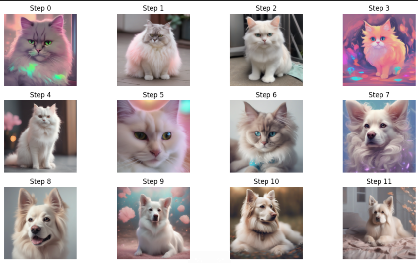
1️⃣ Latent Interpolation Latent interpolation means moving smoothly between two points in latent space. Each point corresponds to a meaningful image after decoding via VAE. This allows smooth transitions like face A → face B, or dog → cat.

2️⃣ VAE Decoding and Non-Linearity The VAE encoder compresses images into latent codes, and the decoder reconstructs them. Both encoder and decoder are deep neural networks — they model complex, non-linear relationships. This lets them capture high-level semantics, not just raw pixels.

3️⃣ Latent Arithmetic You can do math directly in latent space. For example: z_new = z1 + α * (z_text - z1) This moves the image toward a text description — like adding ‘glasses’ or ‘smiling’. This is the basis for text-to-image editing and semantic control.

4️⃣ Interpretable AI Latent space isn’t random — directions correspond to interpretable changes. For instance, certain axes might encode brightness, pose, expression, or object class. By visualizing these effects, we understand how models interpret data.

#VAE+CLIP vs SDXL Interpolation

#Why SDXL Interpolation Works

#1. Text Embeddings Are Aligned with Image Generation

• Stable Diffusion XL (SDXL) is a text-to-image diffusion model. It was trained end-to-end to map text embeddings (from a powerful text encoder) to image latents and then decode them into realistic images.
• When you interpolate between two prompt embeddings (e.g., “a portrait photo” and “a beautiful landscape painting with mountains and a lake”), you are moving smoothly in a semantic space that the model understands.
• The SDXL model’s cross-attention layers were trained to connect these text embeddings to visual features, so any point along the interpolation path corresponds to a meaningful, plausible image.

#2. The Pipeline Handles All Alignment Internally

• The pipe.encode_prompt() method returns all the embeddings (prompt, pooled, and negative) that the model expects for generation.
• By interpolating both prompt_embeds and pooled_prompt_embeds, you ensure the model receives a consistent, valid representation at every step.
• The model’s decoder was trained to turn these latent representations into high-quality images, so the results are always visually meaningful.

---

#Why the Old VAE+CLIP+Projection Approach Failed

#1. No Shared Training or Alignment

• In your old approach, you took a CLIP text embedding and projected it into the VAE latent space using a randomly initialized linear layer.
• The VAE was trained only to encode and decode images, not to understand or reconstruct from random vectors or text projections.
• The CLIP embedding and VAE latent live in different spaces; a random projection does not create a valid image latent.

#2. Out-of-Distribution Latents

• When you interpolate between a real image latent and a random projection of a text embedding, you move into regions of latent space where the VAE decoder has never been trained to produce meaningful images.
• The result: the decoder outputs “garbage”—typically uniform grey, green, or noisy images—because those latents do not correspond to any real image.

---

#Why This SDXL Approach Works—With Example

Imagine:

• SDXL has learned a map:
  “A portrait photo” → latent (looks like a face)
  “A landscape painting” → latent (looks like a landscape)
• Interpolating between these two text embeddings produces latents that are “in-between” the two concepts.
• Because the model was trained to decode any point in this text embedding space into a plausible image, the images transition smoothly from portrait to landscape.

In contrast:

• The VAE+CLIP method is like asking a translator to turn a French poem into Chinese using a dictionary with random words. The result is gibberish.
• SDXL is like using a professional translator who understands both languages and the context, so every “step” in the translation makes sense.

---

#Summary Table

Approach	How It Works	Why It Fails/Succeeds
VAE + CLIP + Linear	Randomly projects text to image latents	Spaces unaligned, decoder not trained; outputs gray/green images
SDXL Interpolation	Interpolates in trained text embedding space; model decodes to image	Model trained for this; every point is valid and meaningful

---

#Key Takeaway

• Text-to-image diffusion models like SDXL are trained to connect text and image spaces.
• Interpolating between prompt embeddings in SDXL works because the model is trained to decode the entire semantic path into plausible images.
• Old VAE+CLIP+projection methods fail because they lack this joint training and alignment.