#Building Faster Multi-Tenant Vector Search: A Deep Dive into Curator

Multi-tenant vector search is hard. Curator achieves 3.4x to 17.3x speedups over traditional IVF by encoding tenant membership directly into the index using bloom filters and hierarchical trees.

---

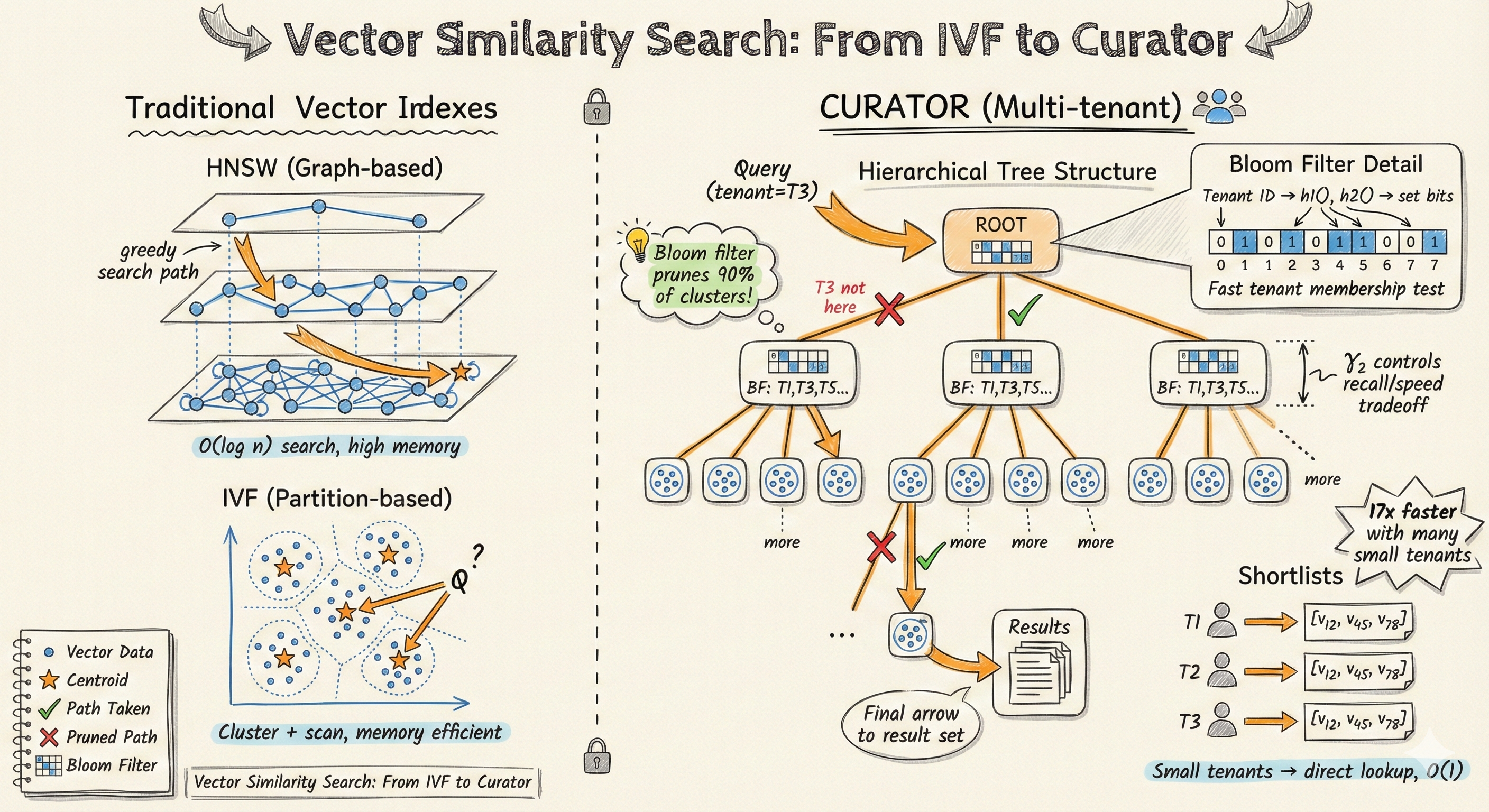
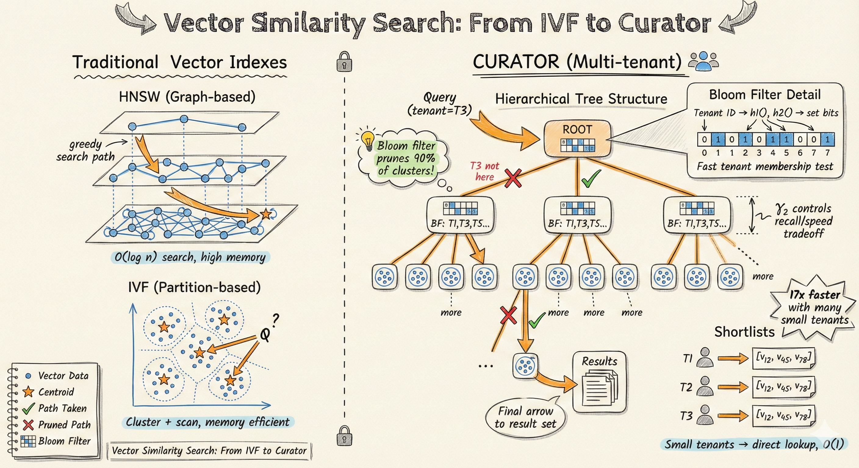
Cover image: Hand-drawn comparison of traditional vector indices (HNSW, IVF) versus Curator’s multi-tenant architecture with bloom filters and hierarchical structure.

---

#Introduction

Vector similarity search powers the AI applications we use every day. When you ask ChatGPT a question and it retrieves relevant context, when Netflix recommends your next show, or when Google finds images similar to your query, vector search is working behind the scenes.

But here is the challenge: most production vector databases serve multiple tenants. Think of a SaaS platform where thousands of customers each have their own documents, embeddings, and access permissions. How do you efficiently search within a single tenant’s data without scanning everyone else’s vectors?

This post explores the vector index landscape, from foundational algorithms like IVF and HNSW to Google’s ScaNN, then dives deep into Curator, a research project that reimagines vector indexing for multi-tenant workloads. We will cover the theory, run experiments, and share real performance numbers.

---

#Part 1: The Vector Index Landscape

#What is Vector Similarity Search?

Given a query vector q and a database of vectors X = {x_1, x_2, ..., x_n}, find the k vectors closest to q:

Top-k = argmin over all x_i in X of ||q - x_i||

This sounds simple, but the curse of dimensionality makes exact search infeasible at scale. With millions of 768-dimensional vectors (typical for text embeddings), brute-force comparison takes seconds per query. Production systems need millisecond latency.

The solution: Approximate Nearest Neighbor (ANN) search. We trade a small accuracy loss for massive speed gains.

#Two Families of Vector Indices

Vector indices fall into two categories: graph-based and partition-based.

---

#Graph-Based: HNSW

Hierarchical Navigable Small World (HNSW) represents vectors as vertices in a proximity graph. Each vertex connects to its nearest neighbors, forming a “small world” network where any two points are reachable in few hops.

Layer 2 (sparse):     A -------- D
                               /
Layer 1 (medium):    A -- B -- C -- D
                      |    |    |    |
Layer 0 (dense):   A-B-E-C-F-G-D-H-I-J

Search algorithm:

1. Start from a fixed entry point at the top layer
2. Greedily move to the neighbor closest to the query
3. When stuck at a local minimum, drop to the next layer
4. At the bottom layer, perform beam search to collect top-k candidates

Complexity: O(log n) search time because the hierarchical structure provides logarithmic “shortcuts.”

Trade-off: High memory usage. Each vector stores an edge list (typically 16-64 neighbors), which can 2-4x the memory footprint compared to just storing the vectors.

---

#Partition-Based: IVF (Inverted File)

IVF divides the vector space into clusters using k-means. Each cluster is represented by its centroid, and vectors are stored in “inverted lists” indexed by their nearest centroid.

Vector Space:                  Index Structure:
                              
   ●●●     ●●●                  Centroid 1: [v3, v7, v12, ...]
  ●★●●   ●●★●●                  Centroid 2: [v1, v5, v18, ...]
   ●●●     ●●                   Centroid 3: [v2, v9, v14, ...]
      ●●●●                      Centroid 4: [v4, v8, v11, ...]
     ●●★●●
       ●●

★ = Cluster centroids
● = Data vectors

Search algorithm:

1. Compute distance from query to all centroids
2. Select the nprobe closest centroids
3. Scan all vectors in those clusters
4. Return top-k from scanned vectors

Complexity: O(n/nlist × nprobe) where nlist is the number of clusters.

Trade-off: More memory-efficient than HNSW (only store centroids + vectors), but typically slower for single queries.

---

#FAISS: The Industry Standard

FAISS (Facebook AI Similarity Search) is Meta’s open-source library implementing dozens of index types. It is the de facto standard for vector search research and powers many production systems.

Key features:

• IVF, HNSW, and hybrid indices
• Product Quantization (PQ) for compression
• GPU acceleration
• Billion-scale search capabilities

FAISS provides the foundation that Curator builds upon, extending IVF with multi-tenant awareness.

---

#Google’s ScaNN: Anisotropic Vector Quantization

ScaNN (Scalable Nearest Neighbors) introduced a clever insight: traditional quantization minimizes reconstruction error uniformly, but for nearest neighbor search, errors parallel to the vector matter more than perpendicular errors.

Traditional quantization:     Anisotropic quantization:
                              
    ●--------○                     ●----○
    (minimize distance)            (minimize parallel error)

By weighting the loss function to penalize parallel errors more heavily, ScaNN achieves 2x better speed-accuracy trade-offs than previous methods. The key innovation: optimize for search accuracy, not compression fidelity.

---

#Part 2: The Multi-Tenant Problem

#Why Multi-Tenancy is Hard

Consider a SaaS vector database serving 1,000 customers:

Traditional approach:

Customer 1: 50,000 vectors
Customer 2: 50,000 vectors
Customer 3: 50,000 vectors
...
Customer 1000: 50,000 vectors
─────────────────────────────
Total: 50 million vectors in one index

When Customer 42 searches for their 10 nearest neighbors:

Standard IVF query:
1. Find nearest clusters → scan 100,000 vectors
2. These vectors belong to ALL customers!
3. Filter to keep only Customer 42's vectors
4. Maybe only 100 vectors survive filtering
5. Hope those 100 contain the true top-10

Problem: 99.9% of work was WASTED!

The fundamental issue: the index has no concept of tenant ownership. It retrieves candidates from all tenants, then filters post-hoc.

---

#How Qdrant Handles Multi-Tenancy

Qdrant implements multi-tenancy through payload filtering and custom sharding:

# Qdrant approach: Store tenant ID in payload
client.upsert(
    collection_name="my_collection",
    points=[
        PointStruct(
            id=1,
            payload={"group_id": "tenant_1"},
            vector=[0.9, 0.1, 0.1], 
        ),
    ],
    shard_key_selector="region_us"
)

# Query with tenant filter
client.search(
    collection_name="my_collection",
    query_filter=Filter(
        must=[FieldCondition(key="group_id", match=MatchValue(value="tenant_1"))]
    ),
    query_vector=[0.1, 0.1, 0.9],
)

Qdrant’s optimization: disable the global HNSW index and build per-tenant indices using payload_m configuration. This helps, but you are still building separate index structures.

---

#How Pinecone Handles Multi-Tenancy

Pinecone uses namespaces for tenant isolation:

# Pinecone approach: One namespace per tenant
index.upsert(
    vectors=[
        {"id": "A", "values": [0.1, 0.1, ...]},
        {"id": "B", "values": [0.2, 0.2, ...]},
    ],
    namespace="tenant1"  # Physical isolation
)

# Query targets only that namespace
index.query(
    namespace="tenant1",
    vector=[0.7, 0.7, ...],
    top_k=3,
)

Namespaces provide physical isolation (each stored separately), making it easy to offboard tenants. The Standard plan supports up to 100,000 namespaces per index.

Both approaches work, but they either:

1. Filter post-query (wasteful scanning), or
2. Maintain separate index structures per tenant (memory overhead)

What if the index itself understood tenants?

---

#Part 3: Enter Curator

#The Key Insight

Curator’s insight is elegant:

“Instead of filtering after search, encode tenant membership INTO the index structure so we can skip irrelevant data DURING search.”

The implementation combines three ideas:

1. Hierarchical IVF tree (not flat clusters)
2. Bloom filters at each internal node (fast tenant membership testing)
3. Per-tenant shortlists for small tenants (bypass the tree entirely)

---

#What is a Bloom Filter?

Before diving into Curator’s architecture, let us understand bloom filters, a probabilistic data structure that answers “Is X in this set?” in O(1) time.

Bloom filter: bit array of size m, initialized to 0

Insert "tenant_5":
  hash1("tenant_5") = 3  →  set bit 3
  hash2("tenant_5") = 7  →  set bit 7
  
  [0, 0, 0, 1, 0, 0, 0, 1, 0, 0]
           ↑           ↑

Query "tenant_5":
  Check bits 3 and 7 → both 1 → "probably yes"

Query "tenant_99":
  hash1("tenant_99") = 2  →  bit 2 is 0 → "definitely no"

Key properties:

• No false negatives: If the filter says “no,” the element is definitely not present
• Possible false positives: If the filter says “yes,” the element might be present
• Space-efficient: A 1% false positive rate needs only ~10 bits per element

For Curator, this means: if a bloom filter says “Tenant T is not in this subtree,” we can skip the entire subtree with confidence.

---

#Curator’s Architecture

                           [ROOT]
                      BF: {all tenants}
                    /         |                     [Node A]      [Node B]      [Node C]
          BF: {1,3,5}    BF: {2,4,6}   BF: {1,2,7}
           /             /             /             [Leaf]  [Leaf] [Leaf] [Leaf] [Leaf]  [Leaf]
        
        
Shortlists (for small tenants):
  Tenant 8: [v12, v45, v78]  ← Only 3 vectors, stored directly
  Tenant 9: [v23, v56, v89, v101]

Components:

1. Hierarchical Tree: Instead of flat IVF clusters, vectors are organized in a tree. Each internal node represents a spatial partition.

2. Bloom Filters: Every internal node has a bloom filter indicating which tenants have vectors in that subtree. Query for Tenant 5? If Node B’s bloom filter says “no,” skip the entire subtree.

3. Shortlists: Tenants with few vectors (fewer than max_sl_size) store their vectors in a direct list. Query = simple scan, no tree traversal needed.

---

#The Search Algorithm

def curator_search(query, tenant_id, k, gamma1, gamma2):
    # Step 1: Check shortlist (small tenants)
    if tenant_id in shortlists:
        return brute_force_search(shortlists[tenant_id], query, k)
    
    # Step 2: Tree traversal with bloom filter pruning
    candidates = []
    priority_queue = [root]
    
    while len(candidates) < gamma2 * k and priority_queue:
        node = pop_closest_to_query(priority_queue)
        
        # Bloom filter check!
        if not node.bloom_filter.might_contain(tenant_id):
            continue  # Skip this entire subtree!
        
        if node.is_leaf:
            candidates.extend(node.vectors_for_tenant(tenant_id))
        else:
            for child in node.children:
                priority_queue.push(child, distance_to_centroid(query, child))
    
    # Step 3: Final ranking
    return top_k(candidates, query, k)

The key parameters:

• gamma1: Controls tree exploration breadth
• gamma2: Candidate set multiplier. Higher = better recall, slower search.
• max_sl_size: Threshold for using shortlists vs tree traversal

---

#Part 4: Experiments

We ran comprehensive experiments comparing Curator against IVF + post-query filtering. All experiments used a RunPod VM with custom-built FAISS including Curator extensions.

#Experiment 1: Simple Benchmark

Setup: 100K vectors, 192 dimensions, 1,000 tenants, 1,000 queries

                        Training    Insert       Query      
Method                  Time        Speed        Latency    QPS
─────────────────────────────────────────────────────────────────
Curator                 1.14s       43,834/s     0.13ms     7,732
IVF+Filter              0.38s       66,252/s     0.62ms     1,609

Result: Curator is 4.8x faster at query time.

Yes, Curator is slower to train (building the tree) and insert (updating bloom filters), but queries are nearly 5x faster. For read-heavy workloads, this trade-off is excellent.

---

#Experiment 2: Parameter Sweep

We tested 81 parameter combinations to understand sensitivity:

Parameter	Values Tested	Impact
nlist	64, 128, 256	Sweet spot around sqrt(n)
gamma1	1, 2, 4	Minimal impact
gamma2	2, 4, 8	Main recall/speed knob
max_sl_size	32, 64, 128	More = faster, slightly less recall

Key finding: gamma2 is THE tuning parameter. Higher gamma2 = scan more candidates = better recall but slower.

gamma2=2:   48,808 QPS,  0.127 recall
gamma2=4:   46,185 QPS,  0.196 recall
gamma2=8:   38,086 QPS,  0.297 recall
gamma2=32:  ~20,000 QPS, 0.83 recall
gamma2=64:  ~10,000 QPS, 1.0 recall

---

#Experiment 3: Workload Analysis

Different tenant distributions stress the index differently:

Workload           │ Curator QPS │ Baseline │ Speedup │ Description
───────────────────┼─────────────┼──────────┼─────────┼────────────────────
Uniform-1000       │      93,661 │    5,427 │ 17.26x  │ 1000 small tenants
Bimodal-100        │      26,745 │    6,494 │  4.12x  │ 20 large + 80 small
Zipf-100           │      24,442 │    6,265 │  3.90x  │ Power-law distribution
SingleDominant     │      24,906 │    6,790 │  3.67x  │ 1 tenant has 50% data
EqualSmall-100     │      19,938 │    5,754 │  3.47x  │ All tenants equal
Uniform-100        │      19,099 │    5,622 │  3.40x  │ 100 equal tenants

Key insights:

1. Curator wins every workload in both speed AND recall
2. Best case: Many small tenants (17x speedup!) because shortlists bypass the tree entirely
3. Worst case: Single dominant tenant (still 3.7x faster!) because bloom filters cannot prune when one tenant is everywhere

---

#Experiment 4: Visualizations

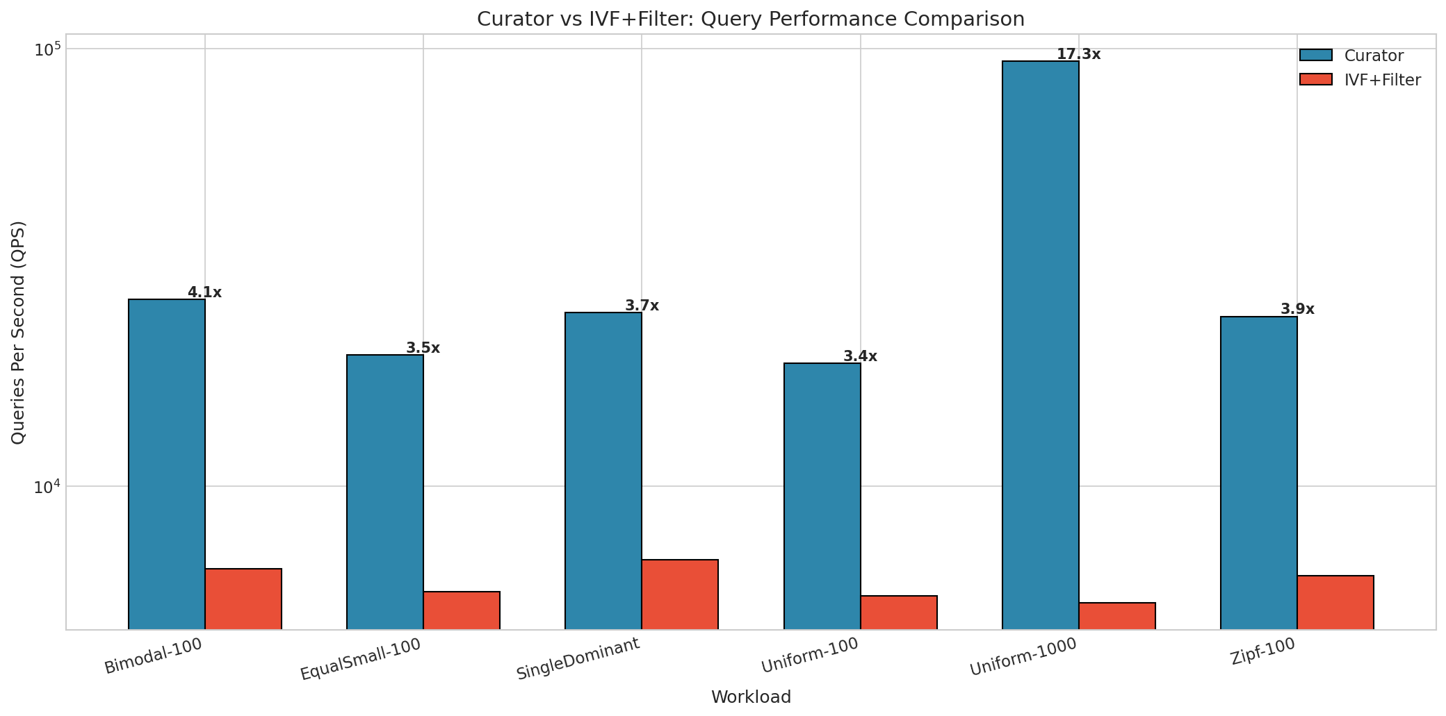Curator consistently outperforms IVF+Filter across all workloads.

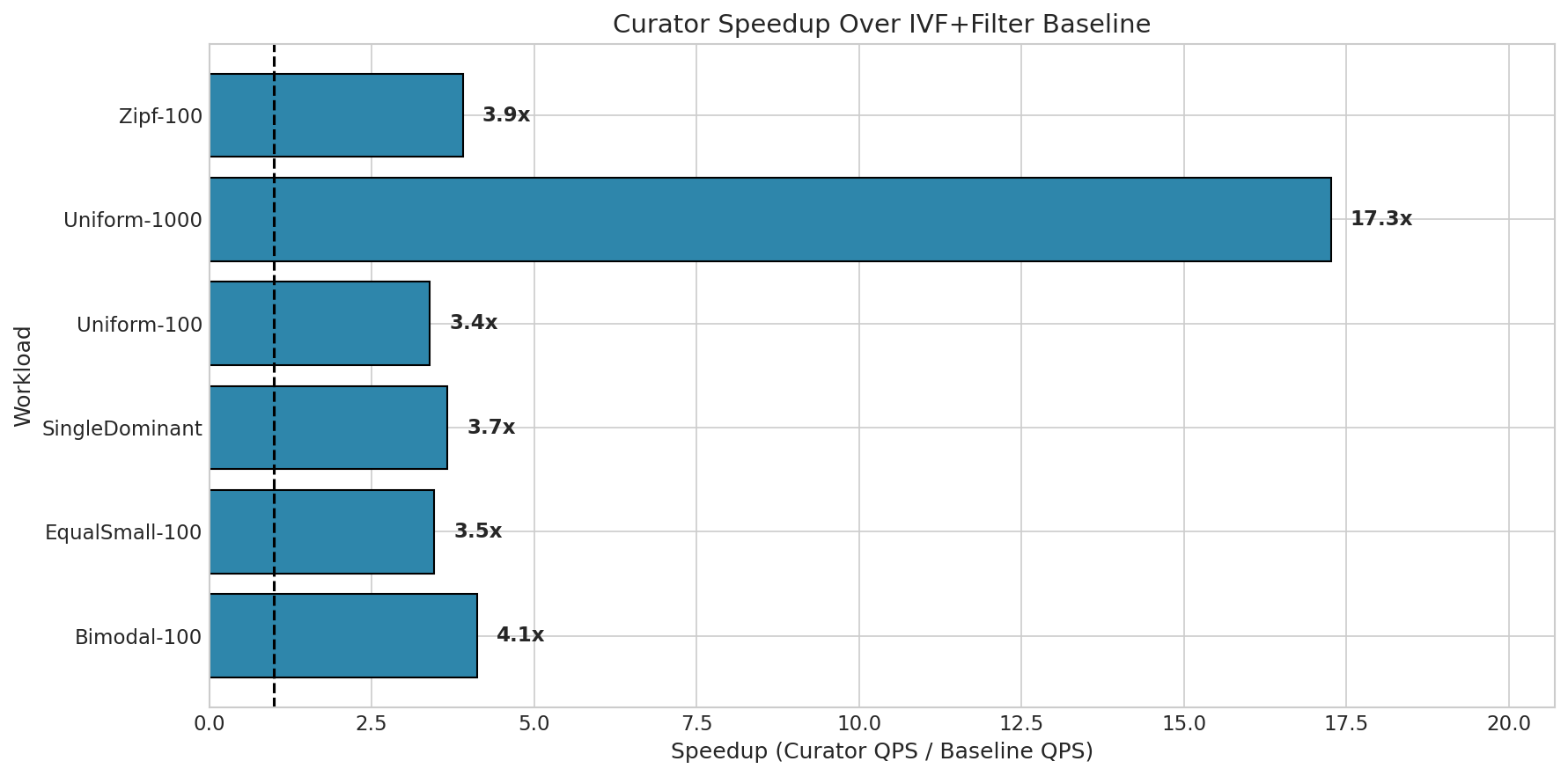Speedup ranges from 3.4x to 17.3x depending on tenant distribution.

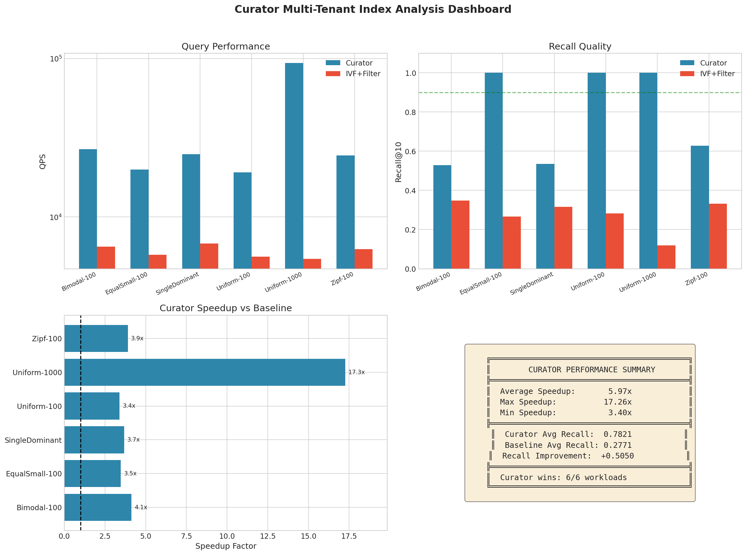Complete performance dashboard showing QPS, recall, and latency comparisons.

---

#Part 5: When to Use Curator

#Curator Excels When:

✅ Many tenants with small data (e.g., 1,000+ users with fewer than 1,000 vectors each)

• Shortlists handle most queries in O(1)
• 17x faster than baseline

✅ SaaS platforms with diverse customers

• Zipf distributions are common (few big, many small)
• Curator adapts to each tenant’s size automatically

✅ Read-heavy workloads

• One-time training overhead amortized over millions of queries
• Insert slowdown acceptable for query speedup

#Curator Struggles When:

⚠️ Single dominant tenant

• If one tenant has 50%+ of data, bloom filters cannot prune
• Solution: Give dominant tenants their own dedicated index

⚠️ Very high recall requirements with clustered data

• Spatially clustered tenant data needs higher gamma2
• Tune parameters or accept lower recall

---

#Part 6: Summary

Index Type	Best For	Multi-Tenant Support
HNSW	Low latency, moderate scale	Post-query filtering
IVF	Large scale, memory-constrained	Post-query filtering
ScaNN	Maximum throughput	Post-query filtering
Qdrant	Managed service	Payload filtering + sharding
Pinecone	Managed service	Namespaces (physical isolation)
Curator	Multi-tenant workloads	Native tenant-aware indexing

#The Bottom Line

Curator proves that tenant-aware indexing can dramatically outperform post-query filtering:

• 3.4x to 17.3x faster than IVF+Filter
• Better recall (not just speed!)
• Automatic adaptation to tenant size via shortlists
• Average 5.97x speedup across diverse workloads

The key innovations:

1. Bloom filters for O(1) tenant membership testing
2. Hierarchical structure for efficient pruning
3. Shortlists for small tenants

For multi-tenant vector databases, the message is clear: build tenant awareness into your index, do not bolt it on after.

---

#References

• FAISS Documentation
• Google ScaNN Announcement
• Qdrant Multi-tenancy Guide
• Pinecone Multi-tenancy Documentation
• Curator Paper: “Curator: Efficient Multi-Tenant Vector Indices” (VLDB 2024)
• HNSW Paper: “Efficient and Robust Approximate Nearest Neighbor Search Using Hierarchical Navigable Small World Graphs”

---

All experiments were run on a RunPod VM with custom FAISS build. Code and results available in the curator repository.

---