Part-1 Reinforcement-Learning - notes

#Objectives

• This post will be the first post in RL series of future posts. In this post, my goal is to share my notes which will help me or anyone to quickly revise the most necessary fundamentals. The next post will be based on my notes from Open AI
• Please check out some code samples checked into my Gitlab related to this blog post. In this post, I may not go really deep in one specific algorithm of RL space. This post shares my notes from one of my favorite teacher, professor Andrew NG, Coursera. Check reference for credits and details.

#RL Intuition

Let me begin with favorite quote and few well known examples of Reinforcement Learning.

| One way to think of why reinforcement learning is so powerful is you have to tell it what to do rather than how to do it. And specifying the reward function rather than the optimal action gives you a lot more flexibility in how you design the system.

Few well known examples of RL applications

• Controlling Robots
• Factory Optimization
• Financial (Stock) Trading
• Playing Games (including video games)

Let us think about autonomous helicopter flying as example. Helicopter can be different states and algorithm (autonomous helicopter) can take any optimal action from available, possible list of actions.

Why not supervised learning?

• One way you could attempt this problem is to use supervised learning. It turns out this is not a great approach for autonomous helicopter flying. But you could say, well if we could get a bunch of observations of states and maybe have an expert human pilot tell us what’s the best action y to take. You could then train a neural network using supervised learning to directly learn the mapping from the states s which I’m calling x here, to an action a which I’m calling the label y here. But it turns out that when the helicopter is moving through the air is actually very ambiguous, what is the exact one right action to take. Do you tilt a bit to the left or a lot more to the left or increase the helicopter stress a little bit or a lot? It’s actually very difficult to get a data set of x and the ideal action y. So that’s why for a lot of task of controlling a robot like a helicopter and other robots, the supervised learning approach doesn’t work well and we instead use reinforcement learning.

Important points

• A key input to a reinforcement learning is something called the reward or the reward function which tells the helicopter when it’s doing well and when it’s doing poorly.
• Concretely for flying the helicopter, whenever it is flying well, you may give it a reward of plus one every second it is flying well. And maybe whenever it’s flying poorly you may give it a negative reward or if it ever crashes, you may give it a very large negative reward like negative 1,000. And so this would incentivize the helicopter to spend a lot more time flying well and hopefully to never crash.
• The key idea is rather than you needing to tell the algorithm what is the right output y for every single input, all you have to do instead is specify a reward function that tells it when it’s doing well and when it’s doing poorly. And it’s the job of the algorithm to automatically figure out how to choose good actions.

#Mars-Rover To Begin With

I like the example of toy Mars_Rover example to explain the core basic of state and action in RL

• Let us assume we are developing reinforcement learning using a simplified example inspired by the Mars rover. In this application, the rover can be in any of six positions, as shown by the six boxes here. The rover, it might start off, say, in disposition into fourth box shown here. The position of the Mars rover is called the state in reinforcement learning, and I’m going to call these six states, state 1, state 2, state 3, state 4, state 5, and state 6, and so the rover is starting off in state 4. Now the rover was sent to Mars to try to carry out different science missions. It can go to different places to use its sensors such as a drill, or a radar, or a spectrometer to analyze the rock at different places on the planet, or go to different places to take interesting pictures for scientists on earth to look at.
• On each step, the rover gets to choose one of two actions. It can either go to the left or it can go to the right. The question is, what should the rover do? In reinforcement learning, we pay a lot of attention to the rewards because that’s how we know if the robot is doing well or poorly.

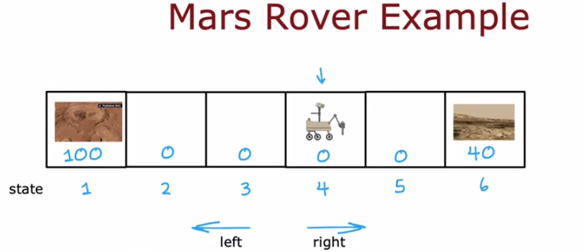
• Let’s look at some examples of what might happen if the robot was to go left, starting from state 4. Then initially starting from state 4, it will receive a reward of zero, and after going left, it gets to state 3, where it receives again a reward of zero. Then it gets to state 2, receives the reward is 0, and finally just to state 1, where it receives a reward of 100. For this application, I’m going to assume that when it gets either state 1 or state 6, that the day ends. In reinforcement learning, we sometimes call this a terminal state, and what that means is that, after it gets to one of these terminals states, gets a reward at that state, but then nothing happens after that.

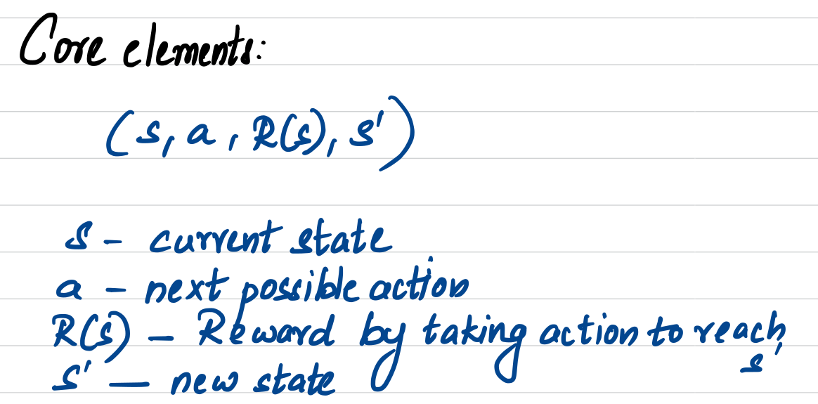
• To summarize, at every time step, the robot is in some state, which I’ll call S, and it gets to choose an action, and it also enjoys some rewards, R of S that it gets from that state. As a result of this action, it to some new state S prime.

• When you learn about specific reinforcement learning algorithms, you see that these four things, the state, action, the reward and next state, which is what happens basically every time you take an action that just be a core elements of what reinforcement learning algorithms will look at when deciding how to take actions.

#Return in RL + Discount Factor

==> In nutshell, Return depends on rewards, rewards depends on actions. Therefore, return depends on actions

how do you know if a particular set of rewards is better or worse than a different set of rewards? Answer is Return which we will see in this section.

Best analogy => if you imagine you have a five-dollar bill at your feet, you can reach down and pick up, or half an hour across town, you can walk half an hour and pick up a 10-dollar bill.Which one would you rather go after? Ten dollars is much better than five dollars, but if you need to walk for half an hour to go and get that 10-dollar bill, then maybe it’d be more convenient to just pick up the five-dollar bill instead.

| The concept of a return captures that rewards you can get quicker are maybe more attractive than rewards that take you a long time to get to.

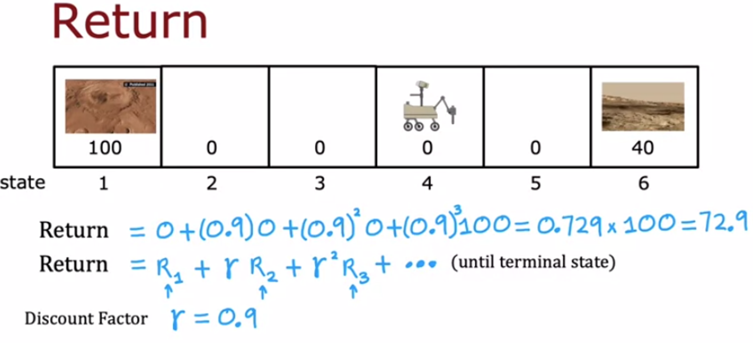
In our Mars Rover example. If starting from state 4 you go to the left, we saw that the rewards you get would be zero on the first step from state 4, zero from state 3, zero from state 2, and then 100 at state 1, the terminal state. The return is defined as the sum of these rewards but weighted by one additional factor, which is called the discount factor. The discount factor is a number a little bit less than 1. Let me pick 0.9 as the discount factor. I’m going to weight the reward in the first step is just zero, the reward in the second step is a discount factor, 0.9 times that reward, and then plus the discount factor^2 times that reward, and then plus the discount factor^3 times that reward. If you calculate this out, this turns out to be 0.729 times 100, which is 72.9.

The more general formula for the return is that if your robot goes through some sequence of states and gets reward R_1 on the first step, and R_2 on the second step, and R_3 on the third step, and so on, then the return is R_1 plus the discount factor Gamma, this Greek alphabet Gamma which I’ve set to 0.9 in this example, the Gamma times R_2 plus Gamma^2 times R_3 plus Gamma^3 times R_4, and so on, until you get to the terminal state

Discount factor Gamma has the effect of making the reinforcement learning algorithm a little bit impatient. Because the return gives full credit to the first reward is 100 percent is 1 times R_1, but then it gives a little bit less credit to the reward you get at the second step is multiplied by 0.9, and then even less credit to the reward you get at the next time step R_3, and so on, and so getting rewards sooner results in a higher value for the total return.

The discount factor (gamma) in reinforcement learning truly influences how patient or impatient an agent is during learning. Here’s how:

#Discount Factor (γ):

• Ranges between 0 and 1.
• Represents the importance an agent places on future rewards compared to immediate rewards.

#Impact on Patience:

• High Gamma (γ closer to 1):

  • The agent values future rewards more heavily.
    • It considers the long-term consequences of its actions.
    • This translates to a more patient agent, willing to forgo smaller immediate rewards for potentially larger rewards later.

• Low Gamma (γ closer to 0):

  • The agent prioritizes immediate rewards.
  • It focuses on the short-term benefits of its actions.
  • This leads to a more impatient agent, favoring smaller rewards now over the possibility of bigger rewards later.

#Example:

Imagine an agent is navigating a maze to find food (reward).

• High Gamma: The agent might take a longer path with scattered food pellets because it anticipates a bigger reward at the end (more patient).
• Low Gamma: The agent might prioritize grabbing the first food pellet it sees, even if it means stopping short of a potentially larger reward (more impatient).

#Choosing the Right Gamma:

• The optimal gamma depends on the specific environment and learning objective.
• For tasks with delayed rewards, a higher gamma is often preferred to encourage the agent to consider long-term benefits.
• However, a very high gamma can make the learning process slow or unstable.
• In some cases, a lower gamma can be useful for initial exploration to help the agent discover valuable states.

#Here’s an additional point to consider:

• Gamma and Learning Rate: The discount factor (gamma) works together with the learning rate (alpha) of the learning algorithm.

  • The learning rate determines how quickly the agent updates its value estimates based on new experiences.
  • A high gamma with a low learning rate can lead to slow learning, while a low gamma with a high learning rate might cause the agent to be too sensitive to immediate rewards and not learn effectively.

By carefully tuning both gamma and the learning rate, we can influence the agent’s patience and achieve optimal learning behavior in a reinforcement learning setting.

• Getting rewards sooner results in a higher value for the total return.

• In financial applications, the discount factor also has a very natural interpretation as the interest rate or the time value of money. If you can have a dollar today, that may be worth a little bit more than if you could only get a dollar in the future. Because even a dollar today you can put in the bank, earn some interest, and end up with a little bit more money a year from now. For financial applications, often, that discount factor represents how much less is a dollar in the future where I’ve compared to a dollar today. Let’s look at some concrete examples of returns. The return you get depends on the rewards, and the rewards depends on the actions you take, and so the return depends on the actions you take.

• Now, this actually has an interesting effect when you have systems with negative rewards. In the example we went through, all the rewards were zero or positive. But if there are any rewards are negative, then the discount factor actually incentivizes the system to push out the negative rewards as far into the future as possible. Taking a financial example, if you had to pay someone $10, maybe that’s a negative reward of minus 10. But if you could postpone payment by a few years, then you’re actually better off because $10 a few years from now, because of the interest rate is actually worth less than $10 that you had to pay today. For systems with negative rewards, it causes the algorithm to try to push out the make the rewards as far into the future as possible. For financial applications and for other applications, that actually turns out to be right thing for the system to do. You now know what is the return in reinforcement learning

#Making Decisions - Policies

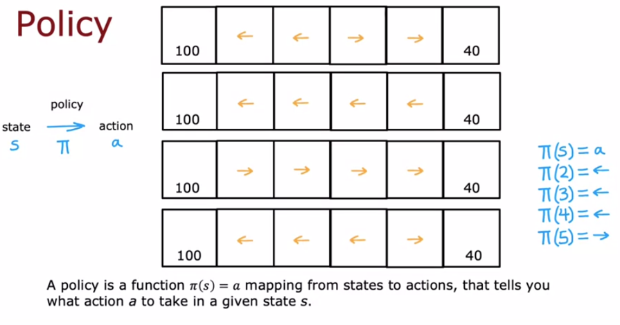
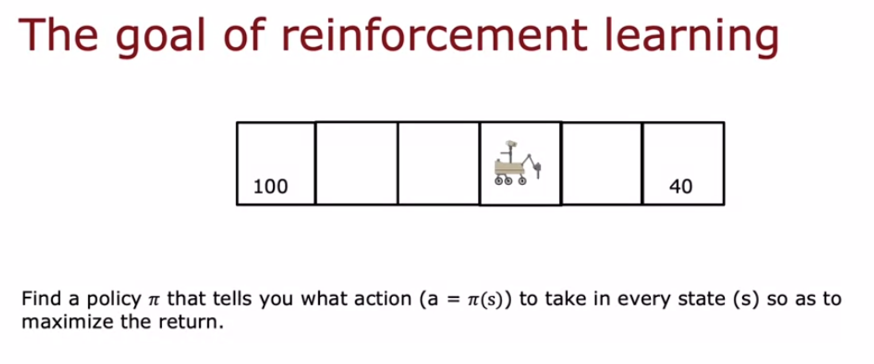
• In reinforcement learning, our goal is to come up with a function which is called a policy Pi, whose job it is to take as input any state s and map it to some action a that it wants us to take. For example, for this policy here at the bottom, this policy would say that if you’re in state 2, then it maps us to the left action. If you’re in state 3, the policy says go left. If you are in state 4 also go left and if you’re in state 5, go right. Pi applied to state S, tells us what action it wants us to take in that state. The goal of reinforcement learning is to find a policy Pi or Pi of S that tells you what action to take in every state so as to maximize the return

Key Terms

• States of reinforcement learning problem
• Set of actions.
• Rewards.
• Discount Factor
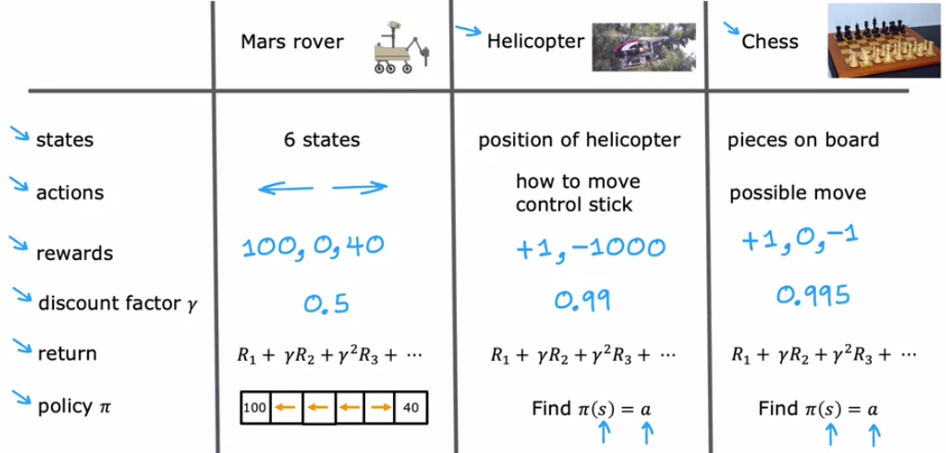
• Rewards + Discount Factor ==> calculate return.
• Policy ==> pick actions so that we can maximize return.

| The job of a reinforcement learning algorithm would be to find some policy Pi of s so that given as input, the position of the helicopter s, it tells you what action to take. That is, tells you how to move the control sticks.

#A Good Summary

#Detailed Recap on Markov

We will talk about Markov in this post, in other posts related to NLP, we will hear the name Markov, in other areas of Baysian inference, we can hear the name Markov again. In the context of RL, before we talk about Markov Decision process, I like to share my notes as a recap about term Markov

#Markov Chain:

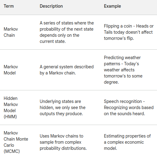
• This is the foundation. A Markov chain is a series of states where the probability of transitioning to the next state depends only on the current state, not the history leading up to it. Imagine flipping a coin - the chance of getting heads next depends only on the current flip, not whether you got heads or tails before.
• Markov chains are used in many applications like modeling random walks, predicting weather patterns (sunny today depends on if it was sunny yesterday), or analyzing text where the probability of the next word depends on the current word.

#Markov Model:

• A Markov model is a more general term for any system that can be described by a Markov chain. It’s basically a system where the future depends only on the present state, not the entire history.
• There are different types of Markov models depending on the nature of the states and transitions (e.g., hidden Markov models).

#Hidden Markov Model (HMM):

• This is a more complex type of Markov model where the underlying states (hidden) are not directly observable. We only see the outputs (emissions) produced by these states.
• Imagine being in a room with hidden weather (sunny/rainy) but you can only see if it’s thundering (emission). An HMM can be used to figure out the hidden weather state based on the observed thunder.
• HMMs are widely used in speech recognition, where the hidden states are the speaker’s vocal tract configurations, and the emissions are the sounds we hear. They are also used in bioinformatics, stock market analysis, and many other fields.

#Markov Chain Monte Carlo (MCMC):

• This is a powerful statistical technique that uses Markov chains to sample from complex probability distributions.
• Imagine having a complicated distribution you want to understand but it’s difficult to calculate probabilities directly. MCMC creates a chain that jumps around the distribution according to certain rules, eventually settling on a representative sample.
• MCMC is used in various scientific fields to analyze data, perform parameter estimation in complex models, and solve optimization problems.

#In-context of RL

Markov Decision Process (MDPs) introduce an additional element: decisions and rewards.

• Markov chains, models, and HMMs deal purely with probabilities of transitioning between states. There’s no concept of an agent making choices or receiving rewards.
• MDPs build on top of Markov chains. They represent situations where an agent can take actions in different states, and these actions influence the transition probabilities and lead to rewards (positive or negative outcomes).

Here’s a breakdown:

• MDPs are for decision-making: Imagine a robot navigating a maze. The robot’s location is a state, and its actions (move left, right, etc.) influence the transitions and lead to rewards (reaching the goal) or penalties (hitting a wall). MDPs help the robot learn the best course of action in each state to maximize its reward.
• Markov chains and models are for understanding sequences: They describe how things evolve over time based on probabilities. They don’t involve making choices or getting rewards.

So, MDPs are a powerful tool for problems where an agent needs to make optimal decisions in an environment with probabilistic transitions and rewards. Markov chains and models are helpful building blocks for understanding the underlying probabilistic nature of the environment.

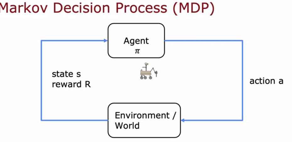
| Above said formalism of a reinforcement learning application actually has a name. It’s called a Markov decision process

| The term Markov in the MDP or Markov decision process refers to that the future only depends on the current state and not on anything that might have occurred prior to getting to the current state. In other words, in a Markov decision process, the future depends only on where you are now, not on how you got here.

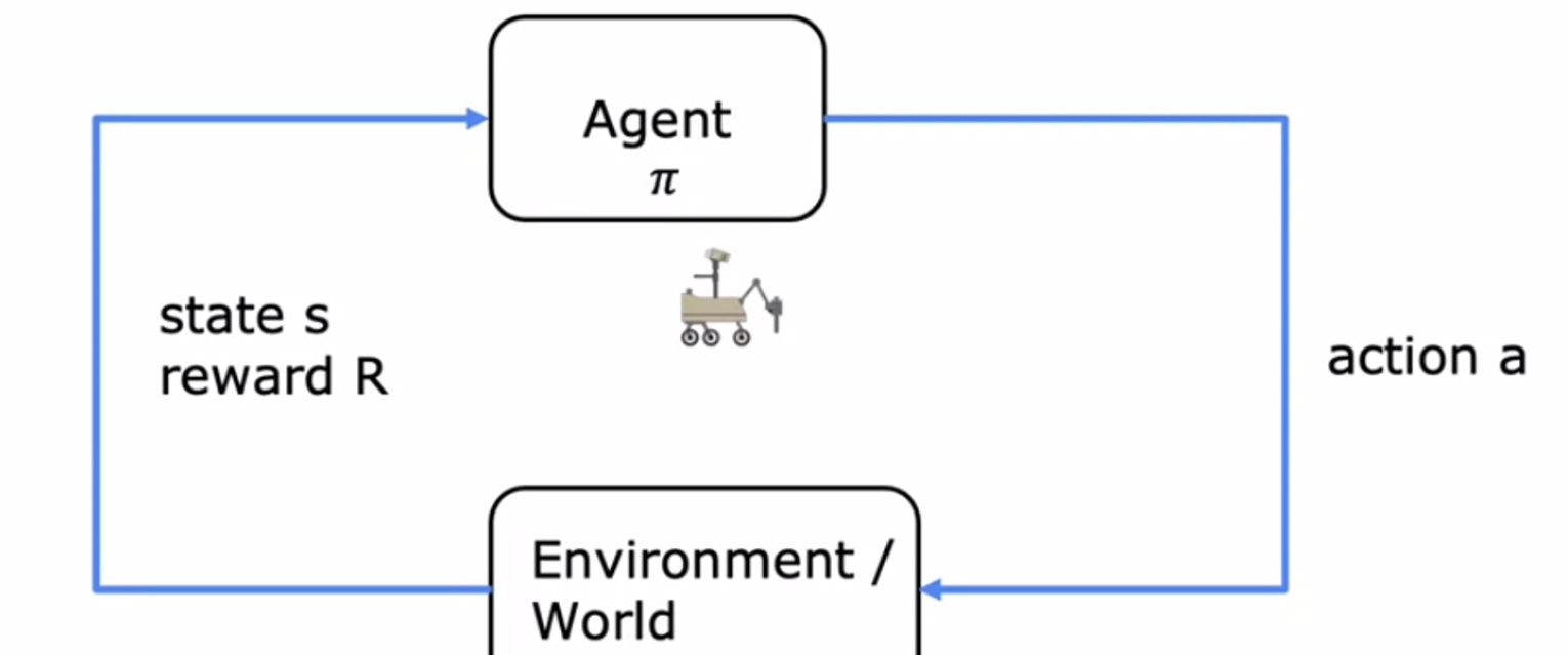
One other way to think of the Markov decision process formalism is that we have a robot or some other agent that we wish to control and what we get to do is choose actions a and based on those actions, something will happen in the world or in the environment, such as our position in the world changes or we get to sample a piece of rock and execute the science mission. The way we choose the action a is with a policy Pi and based on what happens in the world, we then get to see or we observe back what state we’re in, as well as what rewards are that we get.

#State-Action Value Function

---> So far, we have seen state, different action, rewards set for different state, way to calculate return with discount factor ---> We have also seen policy which is a function between s and a, which maximizes the return

| Now we will see Q(s, a) which when calculated for every state and action, then when you are in some state s, look at different actions, pick action a which maximizes Q(s, a), that will turn out as an optimal action

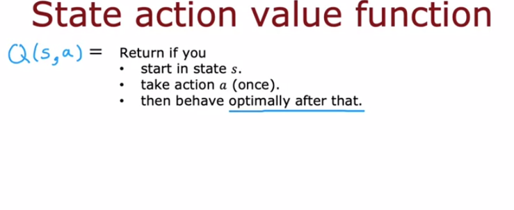
• If you start in that state. S and take the action A just once and after taking action A once you then behave optimally after that. So after that you take whatever actions will result in the highest possible return.

| —> Another important point to pay attention is the circular dependency, where as per the definition of Q(s, a) where you take action once, after that it says follow optimal policy. if you know optimal policy already, what is the need for Q(s, a)

Let us see the way to apply above said definition of Q(s, a) to calculate Q values for each and evevy state. Remember, take action and then follow optimal policy.

For example, at state 2, go right, reach 3. After that follow the directions, so go to state 2 again, then follow the optimal policy to reach the terminal state.

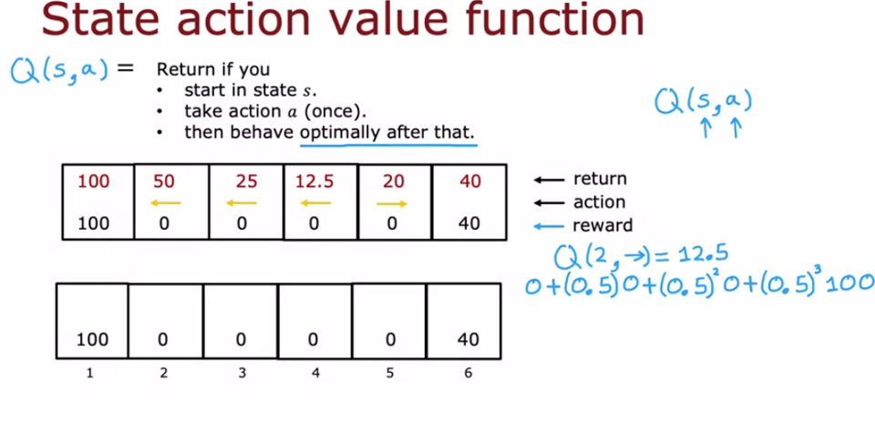
Now, we got different value calculated and initially present which can lead us towards the reinforcement learning process.

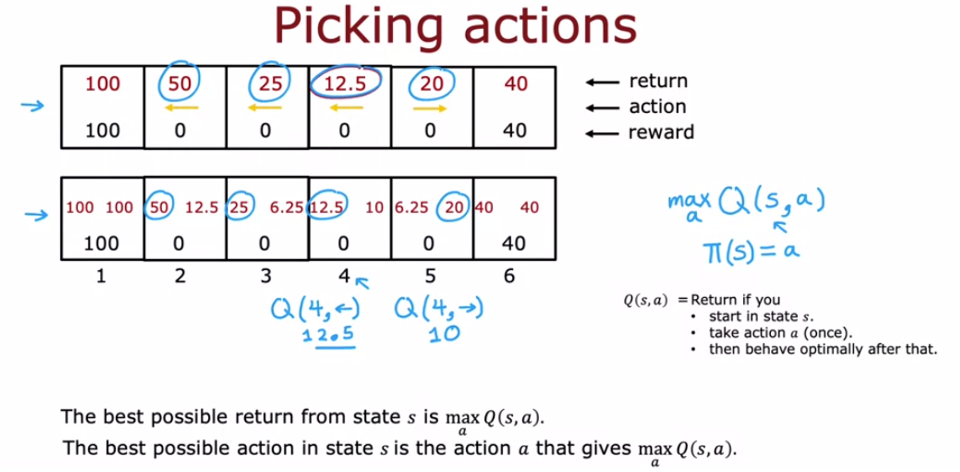
To summarize if you can compute Q of s,a. For every state and every action, then that gives us a good way to compute the optimal policy pi of S. So that’s the state action value function or the Q function.

Also refer to this notebook for sample code to play around, state-action value function code

#Bellman Equation

How do you compute these values Q of S,A? In reinforcement learning, there’s a key equation called the Bellman equation that will help us to compute the state action value function.

The Bellman equation is a fundamental concept in reinforcement learning that captures the relationship between the value of a state and the expected future rewards achievable from that state. It essentially states that the value of a state can be calculated as the immediate reward received by taking an action in that state, plus the discounted value of the next state reached.

V(s) = R(s, a) + γ * V(s')

Where:

- V(s): The value of state s (represents the expected future reward achievable from state s).
- R(s, a): The immediate reward received for taking action a in state s.
- γ (gamma): The discount factor (0 <= γ < 1).
- V(s'): The value of the next state s' reached after taking action a in state s.

#Discount Factor (γ):

• This factor balances the importance of immediate rewards vs. future rewards.
• A higher γ emphasizes future rewards more, encouraging the agent to consider long-term benefits.
• A lower γ prioritizes immediate rewards, making the agent more focused on short-term gains.

#Role in Reinforcement Learning:

• The Bellman equation provides a powerful tool for finding optimal policies (strategies) in an environment.
• By iteratively applying the equation, we can update the value estimates for each state, converging towards the true value of each state under the current policy.
• These value estimates can then be used to improve the policy. For example, the agent can choose actions that lead to states with higher estimated values.

#Example:

Imagine you’re training a robot to navigate a building to find a charging station (reward).

• Let’s say the robot is in a hallway (state s).
• There are two actions possible: a1 (go left) and a2 (go right).
• The immediate reward for each action might be 0 (no reward for movement yet).
• Suppose the robot has already explored and knows the values of the next states:
• If it goes left (s’), it’ll reach a dead end (low value V(s’)).
• If it goes right (s”), it’ll be closer to the charging station (higher value V(s”)).
• Using the Bellman equation, the robot can estimate the value of the current state (s).

V(s) = R(s, a1) + γ * V(s')  // Considering going left (a1)
V(s) = R(s, a2) + γ * V(s'') // Considering going right (a2)

• By comparing the estimated values for both actions, the robot will likely choose to go right (a2) as it leads to a state with a higher expected future reward (closer to the charging station).

In essence, the Bellman equation provides a theoretical foundation for value-based reinforcement learning algorithms. It allows us to iteratively improve our understanding of the environment and make better decisions based on the potential long-term rewards.

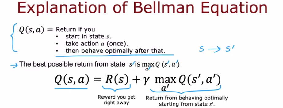
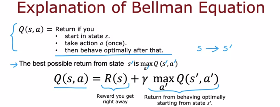
High level intuition ==> the total return you get in the reinforcement learning problem has two parts. The first part is this reward that you get right away, and then the second part is Gamma times the return you get starting from the next state s prime. As these two components together, R of s plus Gamma times the return from the next state, that is equal to the total return from the current state s. That is the essence of the Bellman equation.

#Quick Recap

State-action value function (Q-value function) and a policy are two different but interrelated concepts in reinforcement learning. Here’s how they differ, along with an example:

#Policy (π):

• A policy defines the agent’s behavior in each state.
• It’s a mapping from states (s) to probabilities of taking actions (a).
• Simply put, it tells the agent what action to take in a given situation.

#State-Action Value Function (Q-value function):

• Represents the expected future reward (discounted) of taking a specific action (a) in a given state (s) and following the policy π thereafter.
• It estimates the “goodness” of taking a particular action in a particular state.
• Higher Q-value for an action (a) in state (s) indicates it’s likely to lead to better rewards in the long run.

Analogy:

Imagine you’re an agent navigating a maze to find cheese (reward).

• The policy is like a set of navigation rules you follow. It could be “always go left” or “go towards the strongest cheese smell.”
• The Q-value function is like a map where each maze location shows the expected amount of cheese you’d get if you went left, right, etc., from that spot, considering your current navigation rules (policy).

Here’s how they work together:

• The agent finds itself in a state (e.g., a specific location in the maze).
• The agent consults the policy to determine the action probabilities for that state.
• The agent might also look at the Q-value function to see the estimated rewards for each action in that state.
• Based on the policy and potentially the Q-values, the agent chooses an action (e.g., go left).
• The agent receives a reward (or penalty) and transitions to a new state.
• Over time, the agent can learn and update both the policy (based on successful actions) and the Q-value function (based on experienced rewards).

In short, the policy dictates what the agent does, while the Q-value function helps the agent choose the best action within the policy’s framework. They work together for the agent to learn and improve its behavior in the environment.

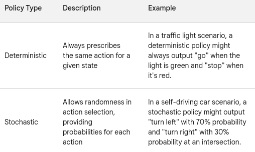
A policy can be either a function that gives a single value (deterministic) or a function that gives a list of action probabilities (stochastic) for a state in reinforcement learning.

• Deterministic Policy: This type of policy always prescribes the same action for a given state. In other words, for any state s, the policy function π(s) will return a single action a. This is like a strict rule-based system where there’s only one clear course of action for each situation.

• Stochastic Policy: This type of policy allows for randomness in the agent’s behavior. The policy function π(s) returns a probability distribution over all possible actions for a given state s. This means the agent might choose different actions from the available options with a certain probability based on that distribution. This can be useful for exploration in uncertain environments where the agent might need to try different things to learn the best course of action.

#Continous State Space

• In the above simplified Mars rover example we used discrete set of states, and what that means is that simplify Mars rover could only be in one of six possible positions. But most robots can be in more than one of six or any discrete number of positions, instead, they can be in any of a very large number of continuous value positions. For example, if the Mars rover could be anywhere on a line, so its position was indicated by a number ranging from 0-6 kilometers where any number in between is valid. That would be an example of a continuous state space, because the position would be represented by a number such as that is 2.7 kilometers along or 4.8 kilometers or any other number between zero and six.

#Deep Reinforcement Learning

• The key idea is that we’re going to train a neural network to compute or to approximate the state action value function Q of s, a and that in turn will let us pick good actions.

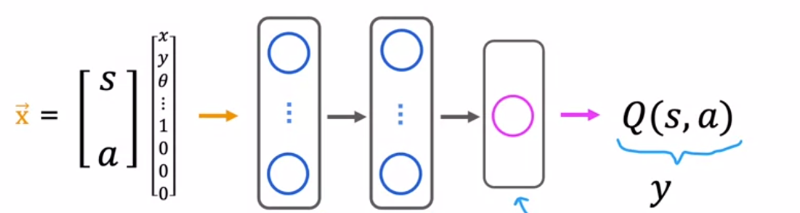
• Remember, reinforcement learning is different from supervised learning, but what we’re going to do is not input a state and have it output an action. What we’re going to do is input a state action pair and have it try to output Q of s, a, and using a neural network inside the reinforcement learning algorithm this way will turn out to work pretty well.

How do you train a neural network to output Q of s, a?

• It turns out the approach will be to use Bellman’s equations to create a training set with lots of examples, x and y, and then we’ll use supervised learning.
• To learn using supervised learning,we need a mapping from x to y, that is a mapping from the state action pair to this target value Q of s, a.

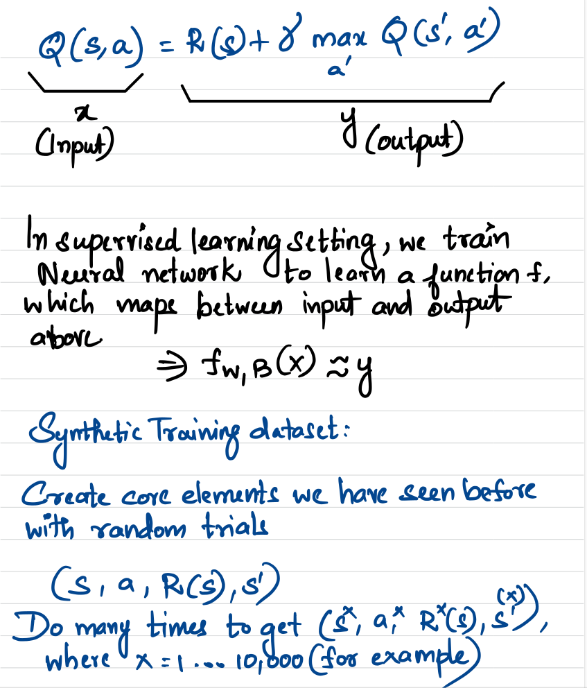
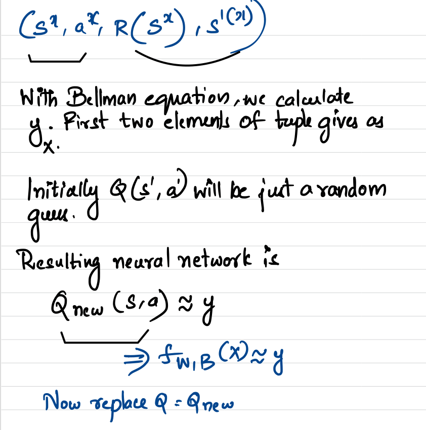
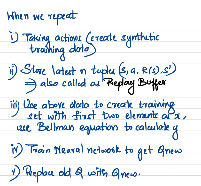
• Now, you may be wondering, where does Q of S’, a’ or Q of S’^1, a’ come from. Well, initially we don’t know what is the Q function. But it turns out that when you don’t know what is the Q function, you can start off with taking a totally random guess.
• The algorithm you just saw is sometimes called the DQN algorithm which stands for Deep Q-Network because you’re using deep learning and neural network to train a model to learn the Q functions. Hence DQN or DQ using a neural network.

#References

• One of my favorite Professor Andrew Ng teachings
• Content from courses from Deep Learning.ai
• And my favorite virtual coach with whom I chat a lot with different prompts, Google Gemini