Prefill, Decode, and the Quiet Third Job: Reviewing vLLM's Guide to Disaggregated Serving
Sources: Taking vLLM Apart: A Practical Guide to Disaggregated Serving by Martin Hickey (IBM Research), September 2026 · framing inspired by Damien Benveniste’s post · refresher material from Inside vLLM by Aleksa Gordić
TL;DR
A single vLLM server does three jobs that get in each other’s way: prefill (compute-bound, sets time to first token), decode (memory-bound, sets how smoothly answers stream), and CPU work around them (templating, tokenizing, parsing, image preprocessing). The vLLM team’s guide shows how to split them: prefill from decode, and the CPU frontend from the GPU box.
Rebuilding the guide’s benchmark from first principles explains its numbers. Its 169 ms tail stutter is one prefill chunk riding in a decode step. Disaggregation removes that stutter but adds a handoff to every first token, and the handoff, not the bandwidth, decides whether it pays.
The payoff is goodput, not throughput. The frontend split matters as much for its interface (an engine that speaks token IDs) as for its cost, and multi-turn KV reuse is a big win that turns into wrong answers when history changes between turns. Includes 9 refreshers, 17 runnable programs, and original figures throughout.
How to read this post
This is a review of a blog post, not a paper, so the right-hand pane works a little differently. The guide is copyrighted, so instead of mirroring it, each linked passage opens the original at the exact sentence. The pane also shows my own figures and, where it helps, the actual vLLM source code. Refreshers are collapsed by default; skip whatever you already know.
Refresher · 6 min read TTFT, ITL, TPOT, percentiles, and goodput The handful of numbers every LLM serving benchmark reports, what each one measures from a user's point of view, and why averages hide what users feel. Skip if You know the difference between ITL and TPOT, and why a p99 matters more than a mean for streaming.
One request, four numbers
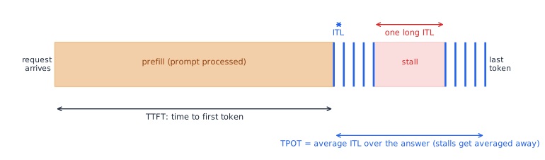
- TTFT, time to first token: from the moment a request arrives until its first output token. Mostly the prefill, plus any queueing. It’s how long a user stares at a blank screen.
- ITL, inter-token latency: the gap between two consecutive output tokens. It decides whether text streams smoothly or stutters.
- TPOT, time per output token: the average ITL across one answer. Benchmarks often use it as the decode-speed target.
- E2E latency: TTFT plus every ITL; the total time until the last token.
The trap is in TPOT. A single 700 ms stall in the middle of a 256-token answer raises its TPOT by less than 3 ms, a rounding error, but the user saw the answer freeze. An average per-token target can be met by an answer that visibly stuttered.
Percentiles: what most users get vs. what some users get
Latency is reported as percentiles over many requests or many tokens. The p50 (median) is the typical experience: half are faster, half slower. The p99 is the experience of the unluckiest 1 in 100. For streaming, the p99 ITL matters most: at 30 tokens per second, a user reading a 300-token answer sees about 300 gaps, so a 1-in-100 stall happens in practically every answer.
Throughput vs. goodput
- Throughput counts everything the server produced: tokens or requests per second, regardless of how long anyone waited.
- Goodput counts only what met its targets. A common definition: the highest request rate at which at least a given share of requests (say 90%) meet both a TTFT target and a decode-speed target.
The two can move in opposite directions. Packing more work onto the same GPUs usually raises throughput while pushing more requests past their latency targets, so goodput falls. A serving design is only better if it’s better at the goodput that matches what your users need, which is why the choice of target (average or worst gap, p50 or p99) is part of the design.
What disaggregation is for: goodput, not throughput
Before any architecture, the objective. The guide is explicit that the pitch isn’t peak throughput: with no latency target, splitting the same GPUs into a prefill pool and a decode pool won’t necessarily move more tokens per second. vLLM’s own documentation is blunter still, stating in capital letters that disaggregated prefill does not improve throughput. What it buys is goodput: the request rate you can sustain while requests still meet both their time-to-first-token target and their decode-speed target. (The refresher above defines all of these terms.)
That reframing changes how to read every benchmark in this post. A design that serves more tokens per second while making users wait longer, or making their answers stutter, has lower goodput. And goodput depends on which targets you pick. To show how much, I measured goodput in my simulator of the guide’s benchmark (built and explained further down) under two different targets:
- An average target: first token within 2 s and TPOT (mean time per output token) at most 30 ms. This is the target in the guide’s own benchmark command.
- A worst-gap target: first token within 2 s, and no single pause between tokens longer than 100 ms, which is roughly when a user notices a stutter.
# Goodput: the request rate you can sustain while requests still meet their latency targets.
# The choice of target matters: an AVERAGE per-token target (TPOT) can hide stalls that a
# worst-gap target exposes.
import numpy as np
from serving_sim import run_requests

SLOS = {
    "A: TTFT <= 2 s and TPOT <= 30 ms (the guide's benchmark)": lambda r: (r[:, 0] <= 2.0) & (r[:, 1] <= 0.030),
    "B: TTFT <= 2 s and no gap > 100 ms (no visible stutter)":  lambda r: (r[:, 0] <= 2.0) & (r[:, 2] <= 0.100),
}
CONFIGS = [("collocated", "collocated", 0.0), ("P/D, 1.3 s transfer", "pd", 1.3), ("P/D, 20 ms transfer", "pd", 0.02)]
RATES = [0.2, 0.4, 0.6, 0.8, 1.0, 1.2, 1.5]

def attainment(rate, mode, tx, slo, seeds=5):
    return np.mean([slo(run_requests(rate, mode, tx, seed=s)).mean() for s in range(seeds)])

def goodput(mode, tx, slo, target=0.9):
    """Highest offered rate at which at least `target` of requests meet the SLO."""
    ok = [r for r in RATES if attainment(r, mode, tx, slo) >= target]
    return max(ok) if ok else 0.0

if __name__ == "__main__":
    for slo_name, slo in SLOS.items():
        print(slo_name)
        print(f"  {'':22s}" + "".join(f"{r:>7.1f}" for r in RATES) + "   goodput (90% met)")
        for name, mode, tx in CONFIGS:
            row = [attainment(r, mode, tx, slo) for r in RATES]
            print(f"  {name:22s}" + "".join(f"{a:>7.0%}" for a in row) + f"   {goodput(mode, tx, slo):.1f} req/s")
        print()
A: TTFT <= 2 s and TPOT <= 30 ms (the guide's benchmark)
0.2 0.4 0.6 0.8 1.0 1.2 1.5 goodput (90% met)
collocated 97% 75% 46% 23% 10% 5% 3% 0.2 req/s
P/D, 1.3 s transfer 0% 0% 0% 0% 0% 0% 0% 0.0 req/s
P/D, 20 ms transfer 100% 99% 95% 88% 73% 41% 11% 0.6 req/s
B: TTFT <= 2 s and no gap > 100 ms (no visible stutter)
0.2 0.4 0.6 0.8 1.0 1.2 1.5 goodput (90% met)
collocated 65% 29% 11% 5% 3% 2% 2% 0.0 req/s
P/D, 1.3 s transfer 0% 0% 0% 0% 0% 0% 0% 0.0 req/s
P/D, 20 ms transfer 100% 99% 97% 92% 87% 76% 37% 0.8 req/s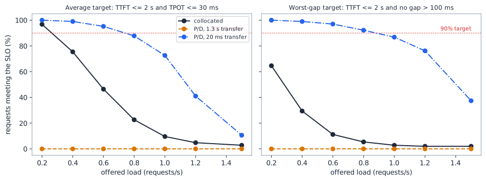
Three things stand out:
- The target decides the verdict. At 0.2 req/s, the collocated server looks healthy under the average target: 97% of requests pass. Under the worst-gap target only 65% do. A long prefill landing mid-answer barely moves an average over 256 tokens, but the user saw the freeze.
- A slow handoff fails everything. With the guide’s measured 1.3 s KV transfer, disaggregated serving meets neither target at any load: every first token arrives just after 2 seconds. The guide reports the same thing.
- A fast handoff wins on both. With a 20 ms transfer, disaggregated serving roughly triples goodput under the average target (0.6 vs 0.2 req/s) and is the only design that sustains any load at all under the worst-gap target.
Keep the worst-gap target in mind. It’s closer to what users experience, and it’s where disaggregation earns its keep.
Setting the stage: one long prompt, two streams
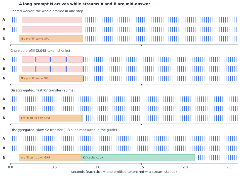
Damien Benveniste’s post on this guide boils the whole trade-off down to one scenario, and it’s the best way in. Two answers, A and B, are streaming to users. Then a third request, N, arrives with a long prompt. N needs a burst of computation before it can say anything; A and B need a small step every few milliseconds to keep their words flowing. Who waits?
Damien lays out three ways to arrange the work: keep everything on one GPU; keep it on one GPU but feed N’s prompt in smaller chunks between A and B’s steps; or compute N’s prompt on a separate GPU pool and copy the result to the decode pool. I simulated all three, the third with both a fast and a slow KV copy, on the hardware the guide benchmarked (Qwen2.5-7B on an NVIDIA L40S), with the costs derived from the model’s size and the GPU’s specs, as explained below:
# Damien Benveniste's scenario, simulated: streams A and B are mid-answer when a new
# 8,192-token prompt N arrives. When does N get its first token, and how long do A and B stall?
from roofline import prefill, decode_step
from serving_sim import step_time, PROMPT

ARRIVE, HORIZON = 0.10, 2.6        # N arrives 100 ms in; simulate 2.6 s

def shared(chunk):
    """One GPU. chunk=None: N's whole prompt runs in one step; otherwise chunked prefill."""
    t, done, tokens = 0.0, 0, {"A": [], "B": [], "N": []}
    while t < HORIZON:
        streams = 2 + (1 if tokens["N"] else 0)
        f, b = decode_step(streams, 2048)
        if t >= ARRIVE and done < PROMPT:
            n = PROMPT - done if chunk is None else min(chunk, PROMPT - done)
            pf, pb = prefill(n, past=done); f += pf; b = max(b, pb); done += n
        t += step_time(f, b)
        tokens["A"].append(t); tokens["B"].append(t)
        if tokens["N"] or done >= PROMPT:
            tokens["N"].append(t)
    return tokens

def disaggregated(transfer_s):
    """Prefill GPU handles N; decode GPU keeps A and B streaming, then adds N after the transfer."""
    f, b = prefill(PROMPT)
    n_ready = ARRIVE + step_time(f, b) + transfer_s
    t, tokens = 0.0, {"A": [], "B": [], "N": []}
    while t < HORIZON:
        joined = t >= n_ready
        f, b = decode_step(2 + joined, 2048)
        t += step_time(f, b)
        tokens["A"].append(t); tokens["B"].append(t)
        if joined:
            tokens["N"].append(t)
    return tokens, n_ready

def summary(name, tokens):
    gaps = [b - a for a, b in zip(tokens["A"], tokens["A"][1:])]
    ttft = tokens["N"][0] - ARRIVE if tokens["N"] else float("nan")
    print(f"{name:34s} N's first token after {ttft*1e3:6.0f} ms | A/B worst stall {max(gaps)*1e3:5.0f} ms")

if __name__ == "__main__":
    summary("shared worker, whole prompt", shared(None))
    summary("shared worker, chunked (2,048)", shared(2048))
    summary("shared worker, chunked (512)", shared(512))
    summary("disaggregated, 20 ms transfer", disaggregated(0.02)[0])
    summary("disaggregated, 1.3 s transfer", disaggregated(1.3)[0])
shared worker, whole prompt N's first token after 731 ms | A/B worst stall 710 ms
shared worker, chunked (2,048) N's first token after 737 ms | A/B worst stall 194 ms
shared worker, chunked (512) N's first token after 763 ms | A/B worst stall 51 ms
disaggregated, 20 ms transfer N's first token after 771 ms | A/B worst stall 24 ms
disaggregated, 1.3 s transfer N's first token after 2053 ms | A/B worst stall 24 msRead the timelines top to bottom:
- Shared worker. N’s whole prompt runs in one step, and A and B freeze for 710 ms: every user watching those answers sees them stop mid-sentence.
- Chunked prefill. The same work, cut into four pieces. A and B now stall four times for about 190 ms each, and with smaller 512-token chunks the worst stall drops to about 50 ms. N’s first token comes slightly later, because its prompt now shares steps with A and B.
- Disaggregated, fast copy. A and B never stall. N’s prompt runs on its own GPU, and its key/value cache crosses to the decode GPU in 20 ms.
- Disaggregated, slow copy. A and B still never stall, but N waits two seconds for its first token. The copy took longer than the prefill itself.
That last row is Damien’s catch, and the guide’s own measurements show it. Everything below is about understanding why each row looks the way it does.
Refresher · 10 min read Attention, model families, and what the KV cache actually stores Queries, keys, and values as a library lookup; who can see whom in encoder, decoder, and encoder-decoder models; and how multi-head, grouped-query, and multi-query attention change the size of the KV cache. Skip if You can explain why decoder-only models cache keys and values, and compute KV bytes per token from a model config.
Attention as a library lookup
Every token, at every layer, is turned into three vectors:
- a query (): what this token is looking for;
- a key (): a label saying what this token contains;
- a value (): the information this token hands over if it’s chosen.
Think of a library. Your question is the query; the catalogue cards are the keys; the books are the values. You compare your question against every card, decide how relevant each one is, and read a weighted mix of the matching books. In math, for token :
Here is how relevant card is to the question.
Here is the head dimension, and the keeps the dot products in a range where the softmax doesn’t saturate. Which the sum runs over, meaning which tokens a token is allowed to look at, is what separates the three model families.
Three families, three masks
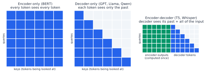
- Encoder-only (BERT, ModernBERT, embedding models). Every token sees every other token, in both directions. The whole input is processed in one pass and nothing is generated token by token, so there’s no “decode” phase at all. Serving these is all prefill.
- Decoder-only (GPT, Llama, Qwen). Each token sees only itself and the tokens before it: a causal mask, the lower triangle. That’s what makes generation possible: the model predicts token from tokens , appends it, and repeats. These models have both phases: a parallel prefill over the prompt, then step-by-step decode.
- Encoder-decoder (T5, Whisper). An encoder reads the input with full attention, once. The decoder then generates causally, and each decoder layer also cross-attends to the encoder’s outputs. The keys and values for that cross-attention are computed once from the encoder and reused at every decoding step.
Almost every chat and agent model served today is decoder-only, so the rest of this refresher focuses on that case.
Why decoder-only models cache K and V
Generation is autoregressive: the probability of an answer to a prompt factors into one prediction per token,
where means all the answer tokens before . So producing tokens takes forward passes. With a causal mask, token ’s key and value depend only on tokens ; nothing that comes later can change them. So once computed, they can be stored and reused. That store is the KV cache.
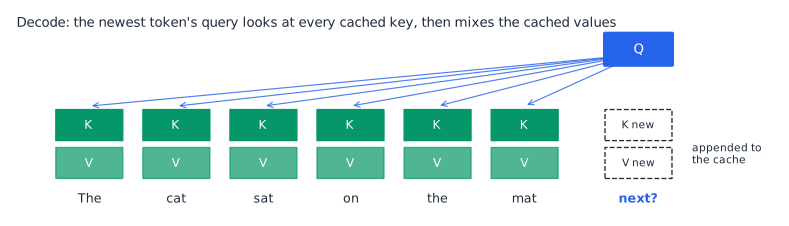
At each decode step, the newest token computes its own , , , compares against every cached key, mixes the cached values, and appends its own and to the cache. Without the cache, every step would recompute the whole prefix. With it, each step does a small amount of new work, but it has to read the entire cache (and all the model’s weights). That is why decode is limited by memory bandwidth, not arithmetic.
Heads: how many K/V pairs per token?
Attention runs in several heads in parallel, each looking for different patterns. The design choice that matters for serving is how many key/value heads there are:

- Multi-head attention (MHA): every query head has its own key and value head.
- Grouped-query attention (GQA): query heads share K/V heads in groups. Llama-3.1-70B has 64 query heads but only 8 K/V heads.
- Multi-query attention (MQA): all query heads share a single K/V head.
- Multi-head latent attention (MLA), used by DeepSeek models, goes further: it caches a compressed latent vector instead of full keys and values.
The KV cache per token is
where the 2 counts one key and one value, is the number of layers, the number of K/V heads, the head dimension, and the bytes per value (2 in BF16). For Llama-3.1-70B in BF16, that’s bytes, or 320 KiB per token. With full multi-head attention it would be eight times larger. GQA is a big part of why serving long contexts is possible at all, and why a KV cache can be moved between GPUs in tens of milliseconds rather than seconds.
The takeaway
- Masks decide which models generate. Encoder-only models are all prefill; decoder-only and encoder-decoder models also decode.
- Causality makes caching valid. A token’s keys and values never change once computed.
- Decode reads everything every step: all the weights and the whole cache. That’s what makes it memory-bound.
- K/V heads set the cache size, and the cache size sets how expensive it is to store, and to move.
Refresher · 8 min read KV caching and prefix caching Why appending to a context is cheap and editing its middle is expensive. Skip if You can explain why prompt caching only works on prefixes, and what re-prefilling costs.
Attention in one equation
At every layer, each token is projected into a query , a key , and a value . In a causal (decoder-only) model, token attends only to itself and the tokens before it:
The property everything else rests on is this: and depend only on tokens through and on position . Tokens that come later never change them. So once computed, they stay valid for as long as nothing before them changes.
The KV cache: compute each token once
Generation has two phases:
- Prefill. The whole prompt is processed in parallel, producing for every prompt token in every layer. This phase is compute-bound.
- Decode. Output is produced one token at a time. Each new token computes only its own and attends over the stored keys and values. This phase is memory-bandwidth-bound.
Storing those keys and values is the KV cache. Without it, every generated token would redo the entire prompt.
The cache is not free. Per token it holds
where the leading 2 counts keys and values, and is the bytes per value (2 in bf16). For Qwen3.6-27B (16 full-attention layers, 4 KV heads, head dimension 256, bf16) that’s bytes, or 64 KiB per token, and 2 GiB for a single 32K-token context. The model’s other 48 layers use linear attention, which keeps a fixed-size state instead of per-token entries; more on that below.
Prefix caching: reuse across calls
An agent resends its entire message list every turn (see the agent-loop refresher). Serving engines exploit this by keeping the KV cache from earlier requests and reusing it whenever a new prompt starts with the same tokens. SGLang does this with a radix tree over token sequences (RadixAttention); vLLM does it with hashed token blocks. Hosted APIs offer the same idea as “prompt caching.”
Reuse stops at the first token that differs. Every later token’s keys and values were computed with the old token in their past, through all the layers above the first, so they are no longer valid:
previous turn : [ A ][ B ][ C ]
append        : [ A ][ B ][ C ][ D ]    reuse A, B, C  ->  prefill only D
edit middle   : [ A ][ B'][ C ]         reuse A        ->  re-prefill B' AND C
edit start    : [ A'][ B ][ C ]         reuse nothing  ->  re-prefill everything
That’s the whole cost story in one picture. Appending is cheap. An edit costs roughly the number of tokens after the edit point, even when those tokens didn’t change. The paper’s cost metric, prefix-reuse FLOPs (§4.1, Eq. 9), counts exactly this. And because hosted-API prompt caching is also prefix-based, the same geometry shows up on your bill.
The position wrinkle: RoPE
Most modern LLMs encode position with rotary embeddings (RoPE): queries and keys are rotated by an angle proportional to their position, . Rotations compose,
so moving a cached key to a new position costs one extra rotation. The position part of a stale cache entry is therefore easy to fix. The content part isn’t: was computed with the old prefix. Suffix Cache Reuse (§4.3) re-rotates surviving keys and accepts the content staleness as an approximation.
Linear-attention layers: a state, not a cache
Linear-attention layers (such as Gated DeltaNet in hybrid models) squeeze the entire history into a fixed-size recurrent state, updated token by token. You can’t delete one token from the middle of such a state. You can only resume from a saved snapshot of the state taken at some earlier point. SGLang saves those snapshots only at request boundaries, which is why hybrid models suffer extra cache misses after edits (Appendix B).
The takeaway
- Keys and values depend on everything before them, so caches are valid only for an unchanged prefix.
- Edit cost scales with how much text comes after the edit, not how big the edit is.
- Positions can be patched cheaply with RoPE. Content can’t, and that tension is exactly what the paper’s serving section is about.
The guide’s opening, sentence by sentence
The guide’s first paragraph makes three claims. Each one deserves unpacking.
Claim 1: one server, three jobs
A plain vllm serve process does three things that get in each other’s way. Two are GPU work: prefill (processing the prompt) and decode (generating the answer). The third is CPU work wrapped around them: turning a chat request into tokens, and tokens back into a structured response.
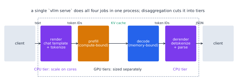
Disaggregated serving cuts that one process into tiers that can be sized, scaled, and placed independently. The guide covers two cuts: prefill from decode, and the CPU work from the GPU box.
Claim 2: splitting prefill from decode works if the KV cache moves fast
The first cut removes prefill from the GPU that serves the streams, so a long prompt can no longer stall them. The cost is a handoff: everything prefill computed, the KV cache, has to reach the decode GPU before N can produce its first token. How big is it? The attention refresher above gives the formula; here it is applied to the guide’s examples:
# How big is the KV cache, and how long does it take to move it?
# Reproduces the numbers quoted in vLLM's disaggregated-serving guide from model configs.

MODELS = {
    #                 layers, query heads, KV heads, head dim
    "Llama-3.1-70B":  (80, 64, 8, 128),
    "Qwen2.5-7B":     (28, 28, 4, 128),
}
BYTES = 2  # bf16

def kv_bytes_per_token(layers, kv_heads, head_dim, bytes_per=BYTES):
    return 2 * layers * kv_heads * head_dim * bytes_per        # 2 = one key + one value

def transfer_ms(total_bytes, gbit_per_s):
    return total_bytes * 8 / (gbit_per_s * 1e9) * 1e3

if __name__ == "__main__":
    for name, (L, hq, hkv, d) in MODELS.items():
        per_tok = kv_bytes_per_token(L, hkv, d)
        mha = kv_bytes_per_token(L, hq, d)                      # if every query head had its own K/V
        print(f"{name}: {per_tok/1024:.0f} KiB per token with {hkv} KV heads "
              f"(would be {mha/1024:.0f} KiB with full multi-head attention, {hq // hkv}x more)")

    per_tok = kv_bytes_per_token(80, 8, 128)
    print(f"\nLlama-3.1-70B, 10k-token prompt: {10_000 * per_tok / 1e9:.2f} GB of KV cache,"
          f" {transfer_ms(10_000 * per_tok, 400):.0f} ms at 400 Gb/s (before any overhead)")

    per_tok = kv_bytes_per_token(28, 4, 128)
    size = 8192 * per_tok
    print(f"Qwen2.5-7B, 8k-token prompt: {size/1e6:.0f} MB of KV cache")
    for label, gbps in [("PCIe 4.0 x16, ~25 GB/s usable", 200), ("400 Gb/s RDMA", 400), ("NVLink-class, ~400 GB/s", 3200)]:
        print(f"  {label:32s} -> {transfer_ms(size, gbps):6.1f} ms of pure copy time")
    print("  measured on the guide's test box (no peer-to-peer) -> about 1,300 ms")
Llama-3.1-70B: 320 KiB per token with 8 KV heads (would be 2560 KiB with full multi-head attention, 8x more)
Qwen2.5-7B: 56 KiB per token with 4 KV heads (would be 392 KiB with full multi-head attention, 7x more)
Llama-3.1-70B, 10k-token prompt: 3.28 GB of KV cache, 66 ms at 400 Gb/s (before any overhead)
Qwen2.5-7B, 8k-token prompt: 470 MB of KV cache
PCIe 4.0 x16, ~25 GB/s usable -> 18.8 ms of pure copy time
400 Gb/s RDMA -> 9.4 ms of pure copy time
NVLink-class, ~400 GB/s -> 1.2 ms of pure copy time
measured on the guide's test box (no peer-to-peer) -> about 1,300 msAll of the guide’s figures check out: 320 KiB per token for Llama-3.1-70B, about 3 GB and roughly 65 ms at 400 Gb/s for a 10k-token prompt, and 470 MB for an 8k-token Qwen2.5-7B prompt. The last line is the important one. On the guide’s test box, that 470 MB took about 1.3 seconds to arrive, roughly 70 times longer than the raw copy should take even over plain PCIe. The guide says so itself: bandwidth doesn’t explain it; overhead around the copy does, including the decode engine only noticing a finished transfer when it checks between its own steps.
So “as long as the KV cache moves fast” has a precise meaning. Disaggregation trades a stall for everyone (the prefill time, landing on every active stream) for a delay for one (the transfer time, landing on the newcomer’s first token). It pays when the transfer is short compared with the stalls it removes. With a 20 ms transfer, that’s an easy win. With a 1.3 s transfer, every request now waits longer for its first word than it would have on a shared GPU.
Claim 3: a CPU-only frontend leaves the engine speaking only token IDs
The second cut is quieter. A model never sees text. Before the GPU does anything, the request’s messages are formatted with the model’s chat template and tokenized into integer IDs. Afterwards, the generated IDs are detokenized back into text, and parsers split that text into the pieces an API returns: the visible answer, the model’s reasoning, and any tool calls. None of that needs a GPU.
The guide’s frontend splits these jobs out into two CPU endpoints around a GPU engine that only takes token IDs in and gives token IDs out:
/render(CPU): chat request → chat template → token IDs./inference/v1/generate(GPU): token IDs → token IDs./derender(CPU): token IDs → text → content, reasoning, and tool calls.
Here are the three hops in miniature, with a toy template, vocabulary, and “model”:
# The three hops of vLLM's split frontend, in miniature:
#   render   (CPU): chat request -> prompt text (chat template) -> token IDs (tokenizer)
#   generate (GPU): token IDs -> token IDs (the only part that needs the model)
#   derender (CPU): token IDs -> text (detokenizer) -> {reasoning, content, tool_calls} (parsers)
# The template, vocabulary and "model" are toys; the shape of the pipeline is the point.
import json, re
from jinja2 import Template

# ---------- render (CPU) ----------
CHAT_TEMPLATE = Template(
    "{% for m in messages %}<|start|>{{ m.role }}\n{{ m.content }}<|end|>\n{% endfor %}"
    "<|start|>assistant\n")

VOCAB = ["<|start|>", "<|end|>", "<think>", "</think>", "<tool_call>", "</tool_call>",
         "Hello", "Hell", "He", "llo", "o", "user", "assistant", "\n", " ", "Weather", " in", " Paris",
         "?", "Need", " the", " tool", ".", '{"name": "get_weather", "args": {"city": "Paris"}}']
VOCAB += [chr(c) for c in range(32, 127) if chr(c) not in VOCAB]       # single characters as a fallback
ID = {tok: i for i, tok in enumerate(VOCAB)}

def tokenize(text):
    """Greedy longest match, a stand-in for a real BPE tokenizer."""
    ids, i = [], 0
    by_len = sorted(VOCAB, key=len, reverse=True)
    while i < len(text):
        tok = next(t for t in by_len if text.startswith(t, i))
        ids.append(ID[tok]); i += len(tok)
    return ids

def render(chat_request):
    prompt = CHAT_TEMPLATE.render(messages=chat_request["messages"])
    return {"token_ids": tokenize(prompt), "max_tokens": chat_request.get("max_tokens", 64)}

# ---------- generate (GPU in real life; here a canned "model") ----------
def generate(gen_request):
    out = ["<think>", "Need", " the", " tool", ".", "</think>",
           "<tool_call>", '{"name": "get_weather", "args": {"city": "Paris"}}', "</tool_call>"]
    return {"token_ids": [ID[t] for t in out]}                          # token IDs in, token IDs out

# ---------- derender (CPU) ----------
def detokenize(ids):
    return "".join(VOCAB[i] for i in ids)

def derender(gen_response, chat_request):
    text = detokenize(gen_response["token_ids"])
    m = re.search(r"<think>(.*?)</think>", text, re.S)                   # reasoning parser
    reasoning = m.group(1) if m else None
    text = re.sub(r"<think>.*?</think>", "", text, flags=re.S)
    calls = [json.loads(c) for c in re.findall(r"<tool_call>(.*?)</tool_call>", text, re.S)]   # tool parser
    content = re.sub(r"<tool_call>.*?</tool_call>", "", text, flags=re.S).strip() or None
    return {"reasoning": reasoning, "content": content, "tool_calls": calls}

if __name__ == "__main__":
    req = {"messages": [{"role": "user", "content": "Weather in Paris?"}]}
    gen_req = render(req)
    print("1. render   ->", len(gen_req["token_ids"]), "token IDs:", gen_req["token_ids"])
    gen_resp = generate(gen_req)
    print("2. generate ->", gen_resp["token_ids"])
    print("3. derender ->", derender(gen_resp, req))

    # Why an engine that speaks token IDs matters: text does not round-trip to the same IDs.
    generated = [ID["He"], ID["llo"]]                                    # what the model actually sampled
    text = detokenize(generated)
    print(f"\nmodel sampled {generated} -> text {text!r} -> re-tokenized {tokenize(text)}")
    print("Same text, different token IDs. An RL trainer that re-tokenizes the text would compute")
    print("log-probabilities for tokens the model never produced.")
1. render -> 11 token IDs: [0, 11, 13, 15, 16, 17, 18, 1, 13, 0, 12]
2. generate -> [2, 19, 20, 21, 22, 3, 4, 23, 5]
3. derender -> {'reasoning': 'Need the tool.', 'content': None, 'tool_calls': [{'name': 'get_weather', 'args': {'city': 'Paris'}}]}
model sampled [8, 9] -> text 'Hello' -> re-tokenized [6]
Same text, different token IDs. An RL trainer that re-tokenizes the text would compute
log-probabilities for tokens the model never produced.The last lines show why an engine that speaks token IDs is more than an efficiency trick. Text doesn’t round-trip to the same token IDs. The model sampled He + llo; re-tokenizing the text Hello gives a single, different token. That matters to:
- Routers, which can pick the replica with the best prefix-cache hit by comparing real token IDs instead of guessing from text.
- RL training, which needs the exact IDs the model produced. My CLM review explains why: GRPO’s importance ratios compare log-probabilities of specific tokens, and re-tokenized text gives you the wrong tokens.
- Reproducibility. My post on why temperature 0 isn’t deterministic covers the other half of that story.
“One server doing three unrelated jobs”
The guide’s first section opens with the symptom anyone running an inference server at load has seen: one long prompt arrives while dozens of answers are mid-stream, and every one of them stutters until that prompt has been processed. The guide blames two phases with almost nothing in common sharing one GPU. Let’s make that precise.
Two phases, and the model families that have them
A decoder-only model (the attention refresher above explains the term) answers in two phases:
- Prefill processes the whole prompt in one parallel pass, filling the KV cache and producing the first output token. Its duration sets the time to first token (TTFT).
- Decode then produces the answer one token per step, each step reading the whole cache. The time between steps is the inter-token latency (ITL): how smoothly the answer streams.
The other families behave differently. An encoder-only model, such as a BERT-style classifier or an embedding model, is all prefill: one pass and done, so it never has this problem. An encoder-decoder model such as Whisper runs its encoder once (prefill-like) and then decodes, so it has both phases, plus cross-attention keys and values computed once from the encoder. vLLM’s separate encoder disaggregation applies the same split-the-phases idea to the encoders of multimodal models.
The math: compute-bound vs memory-bound
Why are the two phases so different? Count the work and the data. A model with parameters does about floating-point operations per token processed: one multiply and one add per weight. In BF16 every weight is 2 bytes, and a forward pass reads every weight from memory once, however many tokens it processes. So for a pass over tokens:
That is, the pass does about FLOPs for every byte it reads: its arithmetic intensity.
A GPU can do a fixed number of operations per second and read a fixed number of bytes per second. For an L40S, that’s about 362 TFLOPS (dense BF16) and 864 GB/s. Their ratio, about 419 FLOPs per byte, is the ridge point. A workload below it waits on memory; a workload above it waits on arithmetic.
- Prefill of an 8,192-token prompt has intensity around 8,000: far above the ridge, compute-bound.
- Decode of a single stream has intensity around 1, and even 64 streams only reach about 50: far below the ridge, memory-bound. Each decode step’s time is essentially the time to read 14 GB of weights at 864 GB/s.
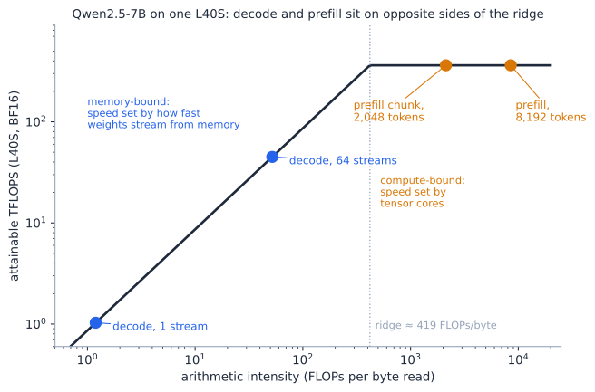
# Why prefill is compute-bound and decode is memory-bound: a roofline model of
# Qwen2.5-7B on one NVIDIA L40S, the setup in vLLM's disaggregated-serving guide.

# Model (Qwen2.5-7B config)
L, D, H, HKV, HD, FF, VOCAB = 28, 3584, 28, 4, 128, 18944, 152064
BYTES = 2                                     # bf16
per_layer = D*D + 2*D*HKV*HD + D*D + 3*D*FF  # q, k+v, o, SwiGLU MLP
N_LAYERS_PARAMS = L * per_layer               # non-embedding parameters
N_HEAD = VOCAB * D                            # output head (untied)

# GPU (L40S datasheet: dense BF16 tensor peak, GDDR6 bandwidth)
PEAK_FLOPS = 362e12
PEAK_BW = 864e9
RIDGE = PEAK_FLOPS / PEAK_BW                  # FLOPs per byte where the roofline bends

def prefill(n_tokens, past=0):
    """FLOPs and bytes to prefill n_tokens that sit after `past` cached tokens."""
    linear = 2 * N_LAYERS_PARAMS * n_tokens + 2 * N_HEAD          # output head only for the last token
    keys = past + (n_tokens + 1) / 2                                 # average keys each new token attends to
    attn = 4 * L * H * HD * n_tokens * keys                          # QK^T and AV, causal
    weights = (N_LAYERS_PARAMS + N_HEAD) * BYTES
    return linear + attn, weights

def decode_step(batch, context):
    """FLOPs and bytes for one decode step: `batch` sequences, each `context` tokens long."""
    linear = 2 * (N_LAYERS_PARAMS + N_HEAD) * batch
    attn = 4 * L * H * HD * context * batch
    weights = (N_LAYERS_PARAMS + N_HEAD) * BYTES                     # read every weight once per step
    kv = batch * context * 2 * L * HKV * HD * BYTES                  # read every cached K and V
    return linear + attn, weights + kv

def roofline_time(flops, bytes_):
    return max(flops / PEAK_FLOPS, bytes_ / PEAK_BW)

if __name__ == "__main__":
    print(f"Qwen2.5-7B: {N_LAYERS_PARAMS/1e9:.2f}B layer params + {N_HEAD/1e9:.2f}B output head")
    print(f"L40S ridge point: {RIDGE:.0f} FLOPs per byte\n")
    print(f"{'workload':34s} {'FLOPs/byte':>10s} {'bound by':>9s} {'ideal time':>11s}")
    rows = [("prefill, 8,192-token prompt", *prefill(8192)),
            ("prefill chunk, 2,048 tokens", *prefill(2048, past=3072)),
            ("decode step, 1 stream @ 8k ctx", *decode_step(1, 8192)),
            ("decode step, 2 streams @ 8k ctx", *decode_step(2, 8192)),
            ("decode step, 64 streams @ 1k ctx", *decode_step(64, 1024))]
    for name, f, b in rows:
        bound = "compute" if f / b > RIDGE else "memory"
        print(f"{name:34s} {f/b:10.0f} {bound:>9s} {roofline_time(f, b)*1e3:9.1f} ms")
    print("\nMeasured in the guide (same GPU and model, low load):"
          "\n  median TTFT, collocated: about 700 ms   (ideal prefill above: ~330 ms -> ~47% of peak FLOPs)"
          "\n  median ITL:              21-24 ms       (ideal decode above:  ~17 ms  -> ~75% of peak bandwidth)")
Qwen2.5-7B: 6.53B layer params + 0.54B output head
L40S ridge point: 419 FLOPs per byte
workload FLOPs/byte bound by ideal time
prefill, 8,192-token prompt 8513 compute 332.5 ms
prefill chunk, 2,048 tokens 2128 compute 83.1 ms
decode step, 1 stream @ 8k ctx 1 memory 16.9 ms
decode step, 2 streams @ 8k ctx 2 memory 17.5 ms
decode step, 64 streams @ 1k ctx 52 memory 20.7 ms
Measured in the guide (same GPU and model, low load):
median TTFT, collocated: about 700 ms (ideal prefill above: ~330 ms -> ~47% of peak FLOPs)
median ITL: 21-24 ms (ideal decode above: ~17 ms -> ~75% of peak bandwidth)These ideal times line up with what the guide measured on that exact setup. Its median TTFT of about 700 ms implies the prefill ran at roughly 47% of the GPU’s peak arithmetic; its median ITL of 21–24 ms implies decode streamed weights at roughly 75% of peak bandwidth. Both are realistic efficiencies, which is a good sign the model is capturing what actually happens.
Why every stream stutters
Now put the two phases on one GPU. A vLLM engine builds each step from a token budget: decodes first, then as much pending prefill as fits (the Inside vLLM capsule below covers this). When a prefill chunk is admitted, the step does both jobs at once, and the step takes as long as its slowest part. A decode step that would take 17 ms now takes as long as the prefill chunk riding along with it. Every stream in the batch waits for it.
How long? A 2,048-token chunk ideally takes 83 ms on an L40S. At the same 47% efficiency the guide’s TTFT implies, that’s about 177 ms.
Now look at the guide’s measurements. At 0.4 requests per second, the collocated server’s p99 ITL jumped from 23 ms to 169 ms. So the p99 stall is almost exactly one 2,048-token prefill chunk. That is what vLLM does by default: for vllm serve on any GPU with less than 70 GiB of memory, which includes the 48 GB L40S, the per-step token budget (max_num_batched_tokens) defaults to 2,048, shared between that step’s decodes and the prefill chunk riding along with them. So the guide’s tail latency is explained from first principles.
“It’s the spike you see the moment concurrency goes up” has a simple reason too. At low load, few prefill chunks happen to coincide with any given stream’s decode steps, so they hide below the 99th percentile. As soon as more than about 1 in 100 decode steps carries a chunk, the p99 jumps from “one decode step” straight to “one prefill chunk.” It doesn’t grow gradually; it switches.
To test the whole picture, I built a small simulator of the guide’s benchmark: two L40S GPUs, 8k-token prompts, 256-token answers, Poisson arrivals, and step times from the roofline model. I calibrated it only on the guide’s low-load medians, then let it predict everything else:
# A first-principles simulation of the guide's benchmark: Qwen2.5-7B on two L40S GPUs,
# ~8k-token prompts, 256 output tokens, Poisson arrivals. Collocated (one engine per GPU,
# chunked prefill mixed with decode) vs disaggregated (one prefill GPU, one decode GPU).
# Step times come from the roofline model; efficiencies are calibrated once to the guide's
# low-load medians (TTFT ~0.7 s, ITL ~22 ms), not to its tail numbers.
import heapq, random
import numpy as np
from roofline import prefill, decode_step, PEAK_FLOPS, PEAK_BW

ETA_C, ETA_B, OVERHEAD = 0.47, 0.75, 0.002     # achieved fraction of peak FLOPs / bandwidth, per-step overhead (s)
PROMPT, OUTPUT, BUDGET = 8192, 256, 2048          # tokens; BUDGET = prefill tokens per collocated step

def step_time(flops, bytes_):
    return max(flops / (PEAK_FLOPS * ETA_C), bytes_ / (PEAK_BW * ETA_B)) + OVERHEAD

def engine(arrivals, mode, transfer_s=0.0):
    """Simulate one engine. mode='mixed' (collocated) or 'decode' (P/D decode pool).
    arrivals: list of (time, req_id) when the request becomes schedulable on this engine.
    Returns dict req_id -> list of token emission times."""
    t, i, waiting, running, emitted = 0.0, 0, [], {}, {}
    arrivals = sorted(arrivals)
    while i < len(arrivals) or waiting or running:
        while i < len(arrivals) and arrivals[i][0] <= t:
            waiting.append([arrivals[i][1], 0]); i += 1          # [req, prompt tokens done]
        if not waiting and not running:
            t = arrivals[i][0]; continue
        flops, bytes_ = 0.0, 0.0
        if running:                                              # decodes go first (as in vLLM's scheduler)
            f, b = decode_step(len(running), PROMPT + 128)
            flops += f; bytes_ += b
        chunk_req = None
        if mode == "mixed" and waiting:                          # fill the rest of the budget with prefill
            req, done = waiting[0]
            n = min(BUDGET - len(running), PROMPT - done)
            f, b = prefill(n, past=done)
            flops += f; bytes_ = max(bytes_, b)
            chunk_req = (req, done + n)
        elif mode == "decode" and waiting:                       # KV already transferred: join the batch
            for req, _ in waiting:
                running[req] = 0; emitted[req] = []
            waiting = []
            continue
        dt = step_time(flops, bytes_)
        t += dt
        for req in list(running):                                # every running stream emits one token
            emitted[req].append(t); running[req] += 1
            if running[req] >= OUTPUT:
                del running[req]
        if chunk_req:
            req, done = chunk_req
            if done >= PROMPT:                                   # prefill finished: first token, start decoding
                waiting.pop(0); emitted[req] = [t]; running[req] = 1
            else:
                waiting[0][1] = done
    return emitted

def run(rate, mode, transfer_s=1.3, n=100, seed=0):
    rng = random.Random(seed)
    t, arrivals = 0.0, []
    for k in range(n):
        t += rng.expovariate(rate); arrivals.append((t, k))
    if mode == "collocated":                                     # two DP ranks, requests alternate between them
        emitted = {}
        for gpu in (0, 1):
            emitted.update(engine([a for a in arrivals if a[1] % 2 == gpu], "mixed"))
    else:                                                        # P/D: prefill GPU (FCFS, whole prompts) -> transfer -> decode GPU
        free_at, ready = 0.0, []
        for at, k in arrivals:
            f, b = prefill(PROMPT)
            start = max(at, free_at); free_at = start + step_time(f, b)
            ready.append((free_at + transfer_s, k))
        emitted = engine(ready, "decode")
    ttft = [emitted[k][0] - at for at, k in arrivals]
    itl = np.concatenate([np.diff(emitted[k]) for k in emitted])
    return np.median(ttft), np.percentile(itl, 50), np.percentile(itl, 99)

if __name__ == "__main__":
    print(f"{'req/s':>5s} | {'collocated':^27s} | {'P/D, 1.3 s transfer':^27s} | {'P/D, 20 ms transfer':^27s}")
    print(f"{'':5s} | {'TTFT':>7s} {'ITL p50':>8s} {'ITL p99':>8s}  " * 3)
    for rate in [0.2, 0.4, 0.6, 1.0, 1.5, 2.0]:
        cells = []
        for mode, tx in [("collocated", 0), ("pd", 1.3), ("pd", 0.02)]:
            res = np.array([run(rate, mode, tx, seed=s) for s in range(5)]).mean(axis=0)
            cells.append(f"{res[0]:6.2f}s {res[1]*1e3:6.0f}ms {res[2]*1e3:6.0f}ms")
        print(f"{rate:5.1f} | " + " | ".join(cells))
req/s | collocated | P/D, 1.3 s transfer | P/D, 20 ms transfer
| TTFT ITL p50 ITL p99 | TTFT ITL p50 ITL p99 | TTFT ITL p50 ITL p99
0.2 | 0.72s 25ms 26ms | 2.04s 25ms 27ms | 0.76s 25ms 27ms
0.4 | 0.75s 25ms 174ms | 2.05s 26ms 29ms | 0.77s 26ms 29ms
0.6 | 0.75s 26ms 184ms | 2.06s 27ms 30ms | 0.78s 27ms 30ms
1.0 | 0.76s 28ms 194ms | 2.28s 29ms 32ms | 1.00s 29ms 32ms
1.5 | 0.76s 31ms 194ms | 4.20s 32ms 33ms | 2.92s 32ms 33ms
2.0 | 0.83s 37ms 194ms | 10.45s 33ms 33ms | 9.17s 33ms 33ms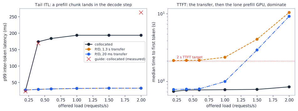
What the simulator reproduces without being told:
- The collocated tail spike at 0.4 req/s, to 174 ms (the guide measured 169 ms).
- Flat P/D tails of 27–33 ms (the guide: 25–52 ms).
- The TTFT penalty of a slow handoff: P/D median TTFT of 2.0 s against 0.7 s collocated (the guide: 2.2 s vs 0.7 s).
What it adds: with 8k prompts, one prefill GPU saturates at about 1.4 requests per second (each prompt takes about 0.7 s), and beyond that TTFT explodes even with a fast transfer. One prefiller per decoder is the wrong ratio for this workload, which is the guide’s “size each pool for its own load” point made concrete.
Where it falls short: the guide’s collocated p99 keeps climbing to 263 ms at 2 req/s, while mine plateaus at about 194 ms. My model lets only one prompt prefill per step and ignores queueing effects that make tails worse at high load.
The third job: CPU work on a GPU box
The guide’s third job is the one people miss: everything that turns requests into tokens and tokens into responses. Five pieces, each pure CPU work:
- Chat templating formats the conversation (roles, system prompt, tool definitions) into the exact prompt string the model was trained on.
- Tokenization turns that string into token IDs.
- Detokenization turns generated IDs back into text, incrementally while streaming.
- Reasoning parsing separates a reasoning model’s thinking from its answer.
- Tool-call parsing extracts structured function calls from the generated text.
Per request this is cheap: the guide measured about 15 ms of CPU to template and tokenize a 9,000-token chat prompt, and one render server handled 73 requests per second on just over one core. The point isn’t that it’s expensive; it’s that you’re running it on a machine you rent for its GPUs, and it competes with the engine’s own CPU-side work.
There’s one place where it does get expensive, and the guide is candid about it: streaming through a parser on a stateless render tier. The tier keeps nothing between chunks, so (as of vLLM v0.31.0; v0.30.0 simply refused to stream through a parser) every streamed chunk carries the output token history in stream_state, and the tier rebuilds the parser and replays that history before parsing the new tokens. Some parsers also rescan all the accumulated text on every call. Count the work:
# Why streaming derender with a parser gets expensive (the guide's "What's still left" section).
# A stateless render tier keeps nothing between chunks, so for every streamed chunk it receives the
# whole token history, rebuilds the parser, and replays the history through it. Parsers such as
# Hermes rescan the accumulated text on each call. Count the character work for n output tokens.

def stateful(n, chars_per_token=4):
    return sum(chars_per_token for _ in range(n))                         # parse each new token once

def stateless_replay(n, chars_per_token=4, rescan=True):
    work = 0
    for chunk in range(1, n + 1):                                         # one token per streamed chunk
        for replayed in range(1, chunk + 1):                              # replay the whole history
            work += replayed * chars_per_token if rescan else chars_per_token
    return work

if __name__ == "__main__":
    print(f"{'output tokens':>13s} {'stateful':>12s} {'replay':>14s} {'replay + rescan':>17s}")
    prev = None
    for n in [250, 500, 1000, 2000, 4000]:
        a, b, c = stateful(n), stateless_replay(n, rescan=False), stateless_replay(n)
        growth = f"  (x{c/prev:.1f} when n doubles)" if prev else ""
        print(f"{n:13,d} {a:12,d} {b:14,d} {c:17,d}{growth}")
        prev = c
    prompt, output = 100_000, 1_000
    print(f"\nprompt token IDs resent with every chunk: {prompt:,} prompt vs {output:,} output tokens "
          f"-> the prompt is {prompt / (prompt + output):.0%} of each request body")
output tokens stateful replay replay + rescan
250 1,000 125,500 10,542,000
500 2,000 501,000 83,834,000 (x8.0 when n doubles)
1,000 4,000 2,002,000 668,668,000 (x8.0 when n doubles)
2,000 8,000 8,004,000 5,341,336,000 (x8.0 when n doubles)
4,000 16,000 32,008,000 42,698,672,000 (x8.0 when n doubles)
prompt token IDs resent with every chunk: 100,000 prompt vs 1,000 output tokens -> the prompt is 99% of each request bodyReplay alone makes the work quadratic in the output length; with a parser that rescans its accumulated text on each call, every doubling of the output multiplies the work by eight: the O(n³) the guide describes. A long reasoning trace makes it bite, and the guide measured roughly nine times the CPU of in-process parsing at matched load. Statelessness is what lets any render replica handle any chunk; the fix that keeps it is caching parser state, which the vLLM team says is scheduled. Until then, the guide’s advice stands: give the render tier more workers than the default of one.
Capsule · 9 min read Capsule: Inside vLLM, how one engine mixes prefill and decode Aleksa Gordić · Read the original A guided summary of Aleksa Gordić's 'Inside vLLM: Anatomy of a High-Throughput LLM Inference System': the engine step, the scheduler's token budget, paged KV blocks, chunked prefill, and how disaggregated P/D plugs in. Skip if You know what happens inside one vLLM engine step, and what a KV connector does.
The source
Inside vLLM: Anatomy of a High-Throughput LLM Inference System by Aleksa Gordić (September 2025, originally on his own site) is the best walk-through of vLLM’s V1 engine I know. Its analysis is pinned to a commit from August 2025, so some names may have changed since; the ideas haven’t. Here is the part you need for disaggregation, in my words.
One engine, one loop
An engine repeatedly calls step(), and each step has three stages:
- Schedule: choose which requests run in this step, and how many tokens each gets.
- Forward pass: run the model once over all of those tokens, then sample.
- Postprocess: append the sampled tokens, detokenize, check stop conditions, and free the KV blocks of finished requests.
Everything that matters for this post happens in stage 1.
The scheduler’s token budget
The scheduler treats the two kinds of work very differently:
- Decode requests (already running) need one new token each, plus a few more when speculative decoding is on. The scheduler handles these first.
- Prefill requests (waiting) need all of their prompt tokens processed. They go second, into whatever room is left in the step’s token budget.
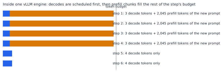
Since the V1 engine, both kinds can share a single step. The forward pass flattens every request in the batch into one long “super-sequence,” and positions plus attention masks keep each request looking only at its own tokens. That’s continuous batching: requests join and leave between steps, with no padding.
Chunked prefill caps how many prompt tokens one request may take in a step, so a long prompt is processed over several steps instead of monopolizing one. A prompt of three chunks needs at least three steps, and its first output token is sampled only in the last one.
Paged KV memory
The KV cache is stored in fixed-size blocks, 16 tokens each by default, handed out from a pool of free blocks. For a standard transformer layer, one block occupies
where is the block size in tokens, the number of KV heads, the head dimension, and the bytes per value. Each request owns a list of blocks rather than one contiguous region, which is what lets thousands of requests of different lengths share GPU memory without fragmentation. Prefix caching builds on the same blocks: full blocks are hashed (each hash chained to the previous block’s), so a new request whose prompt begins with already-cached blocks reuses them instead of recomputing them.
Where disaggregated P/D plugs in
Prefill is compute-bound and decode is memory-bound, so the source frames P/D as running prefill instances and decode instances, sized to the live request mix, with KV caches flowing from one to the other. The piece that moves them is a KV connector, created twice, once inside the scheduler and once inside each worker. Its lifecycle in a step:
- Lookup. While scheduling a waiting request, the scheduler asks the connector how many of its tokens already have KV available externally. Prefill always gets 0; decode may get a hit.
- Bookkeeping. After allocating blocks, the scheduler records which requests will load or save KV, and builds connector metadata for the step.
- Load before, save after. The forward pass runs inside a context manager. On entry, decode starts loading external KV into its paged blocks; on exit, prefill waits until its KV has been saved.
The source illustrates this with a simple shared-storage connector (a local filesystem standing in for a KV service). Production connectors such as NIXL move the blocks over RDMA or GPU-to-GPU links instead. The lifecycle is the same.
Why this matters for the post
In a collocated engine, decode and prefill share every step: decodes go first, but if a prefill chunk is admitted, the whole step, decodes included, takes as long as that chunk. That’s the mechanical reason streams stutter when long prompts arrive. Disaggregation removes the prefill chunk from the decode engine’s steps entirely; the connector is the price.
“Disaggregation is the obvious response”
Having shown one process doing three unrelated jobs, the guide’s conclusion is almost a tautology: stop making one process do all of it. The Inside vLLM capsule above shows what that looks like inside the engine. You run separate prefill and decode instances, sized to the request mix, and a KV connector loads the cache into the decode engine’s paged memory before its forward pass, and saves it from the prefill engine after its own.
That connector is where both the benefit and the risk live. The benefit is the flat tail in the simulator: decode steps never carry a prefill chunk. The risk is the handoff: its size is set by the attention design (GQA keeps it small), its speed by the link between the pools, and its latency lands on every single first token.
The dimensions: what crosses the cut
The guide’s next section lists the places where vLLM can split the work. All of them share one question: when you cut the model in two, what has to cross the wire, how big is it, and how often?
The KV cache, dissected
Prefill and decode run as two separate instances, and the only thing that passes between them is the KV cache: the attention keys and values for every prompt token, which decode needs before it can emit anything. The guide’s numbers are worth taking apart one piece at a time, using the attention refresher from earlier.
What exactly is stored. Every layer of the model keeps two vectors for each prompt token and each key/value head: a key (what this token contains, used to decide relevance) and a value (what the token hands over when it’s attended to). So a prompt’s KV cache is a block of numbers with five dimensions:
| Dimension | Symbol | Llama-3.1-70B |
|---|---|---|
| Layers | 80 | |
| Keys and values | 2 | |
| KV heads per layer | 8 | |
| Numbers per head | 128 | |
| Prompt tokens | 10,000 |
Multiply the five together and you have the count of numbers in the cache. Multiply by the bytes each number takes, (2 in BF16), and you have its size. It’s the attention refresher’s bytes-per-token formula, times tokens:
vLLM stores it in pages of 16 tokens per layer (the Inside vLLM capsule covers this), which is also the unit the connectors move.
Why decode can’t start without it. Decode’s very first step computes the newest token’s query at layer 1 and compares it against every prompt token’s key at layer 1, then does the same at layer 2, and so on up the stack. Without all layers of keys and values, there’s nothing to attend to. The only alternative is recomputing them, which means doing the prefill again.
Why it’s big. Plug in the Llama-3.1-70B column with : each token costs bytes, or 320 KiB. A 10,000-token prompt hands decode about 3.3 GB, which takes roughly 65 ms at a 400 Gb/s line rate before any overhead.
Why “all of it lands on TTFT” is only half true. The transfer lands on the first token if it starts after prefill finishes. But prefill produces the cache one layer at a time, and each layer’s keys and values are final as soon as that layer is done. A connector can ship layer 1’s KV while the GPU computes layer 2, and so on. Two numbers make the case:
# Two questions about moving the KV cache from prefill to decode:
#  1. How much bandwidth does it really need?  (Big in bytes, small relative to the compute that makes it.)
#  2. How much of the transfer must land on TTFT?  (All of it if sent after prefill; ~one layer's worth if
#     streamed layer by layer while prefill computes the next layer, as fabric-lib does.)
from kv_calculator import kv_bytes_per_token

def required_gbps(params, kv_per_token, achieved_tflops):
    """Bandwidth needed to ship KV as fast as prefill produces it."""
    tokens_per_s = achieved_tflops * 1e12 / (2 * params)       # ~2 FLOPs per parameter per token
    return tokens_per_s * kv_per_token * 8 / 1e9

def exposed_transfer_ms(tokens, layers, kv_per_token, link_gbps, prefill_ms, layerwise):
    total_ms = tokens * kv_per_token * 8 / (link_gbps * 1e9) * 1e3
    if not layerwise:
        return total_ms                                         # everything waits until prefill finishes
    per_layer_xfer, per_layer_compute = total_ms / layers, prefill_ms / layers
    # each layer's KV ships while the next layer computes; only the excess (and the last layer) is exposed
    return max(0.0, per_layer_xfer - per_layer_compute) * (layers - 1) + per_layer_xfer

if __name__ == "__main__":
    llama = dict(params=70.6e9, kv=kv_bytes_per_token(80, 8, 128), layers=80)
    qwen = dict(params=7.07e9, kv=kv_bytes_per_token(28, 4, 128), layers=28)

    print("1. Bandwidth needed to keep up with prefill")
    for name, m, tflops, gpu in [("Llama-3.1-70B", llama, 8 * 450, "8x H100 at ~45% of BF16 peak"),
                                 ("Qwen2.5-7B", qwen, 170, "1x L40S at ~47% of BF16 peak")]:
        print(f"  {name:14s} on {gpu:30s}: {required_gbps(m['params'], m['kv'], tflops):6.1f} Gb/s")
    print("  (a single 400 Gb/s NIC is 400 Gb/s)\n")

    print("2. How much of the transfer lands on TTFT (10k-token prompt, Llama-3.1-70B, one 400 Gb/s link)")
    prefill_ms = 2 * llama["params"] * 10_000 / (8 * 450e12) * 1e3
    for layerwise in (False, True):
        e = exposed_transfer_ms(10_000, llama["layers"], llama["kv"], 400, prefill_ms, layerwise)
        label = "streamed layer by layer" if layerwise else "sent after prefill    "
        print(f"  {label}: {e:6.1f} ms added to TTFT   (prefill itself: ~{prefill_ms:.0f} ms)")
1. Bandwidth needed to keep up with prefill
Llama-3.1-70B on 8x H100 at ~45% of BF16 peak : 66.8 Gb/s
Qwen2.5-7B on 1x L40S at ~47% of BF16 peak : 5.5 Gb/s
(a single 400 Gb/s NIC is 400 Gb/s)
2. How much of the transfer lands on TTFT (10k-token prompt, Llama-3.1-70B, one 400 Gb/s link)
sent after prefill : 65.5 ms added to TTFT (prefill itself: ~392 ms)
streamed layer by layer: 0.8 ms added to TTFT (prefill itself: ~392 ms)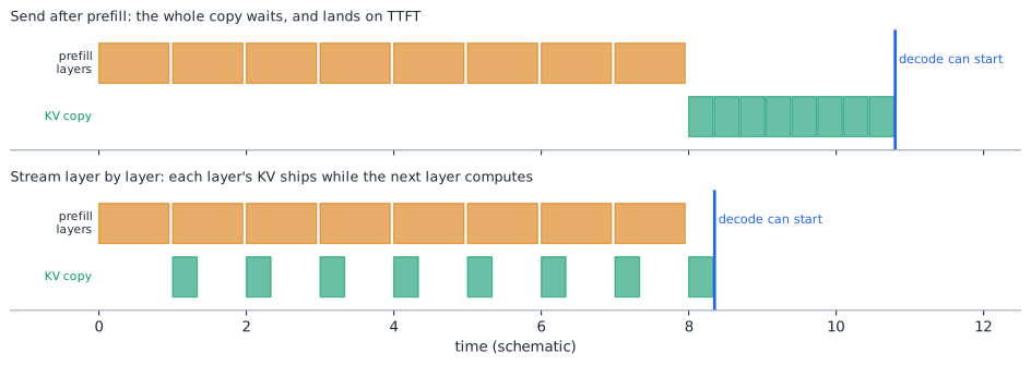
The KV cache is large in bytes but small relative to the compute that produces it. Even an 8-GPU Llama-70B prefill only needs about 67 Gb/s to ship its KV as fast as it makes it, a sixth of one NIC. Streamed layer by layer, only the last layer’s share is exposed: under 1 ms instead of 65 ms. Perplexity’s fabric-lib paper reports exactly this in production. For Qwen3-235B with layer-by-layer transfers, at 8K and 16K tokens each layer’s transfer took about 1.0 and 1.6 ms against 4.6 and 9.9 ms of compute, so the transfer hid behind computation, and most of their small TTFT overhead came from an extra decode pass rather than the copy.
So the guide’s 1.3 s handoff isn’t a law of physics. It’s what happens when the copy waits for prefill to finish, goes through a slow path, and is only noticed when the decode engine next checks.
The KV connector, briefly. In vLLM, the component that moves all this is a KV connector. The documentation lists a range of them:
- NIXL, for RDMA and GPU-to-GPU transfers;
- Mooncake and LMCache, which also offer shared KV stores;
- MoRI-IO, for AMD GPUs;
- an offloading connector that spills KV to CPU memory;
- a MultiConnector that chains several of the above.
Every process gets its own connector instance:
- A scheduler-side connector decides which requests need KV loaded or saved this step.
- Worker-side connectors do the actual copies; the interface lets them work layer by layer alongside the attention computation, though vLLM’s NIXL connector doesn’t use that hook and transfers after prefill finishes.
The docs also name the abstractions you’d build a new one from: a pipe that only sends and receives tensors, and a lookup buffer with database-like insert and select operations.
RDMA in two lines. Remote Direct Memory Access lets a network card read or write another machine’s memory, including GPU memory via GPUDirect, without involving either machine’s CPU or operating system on the data path. That’s how KV caches move at 400 Gb/s with microsecond latencies instead of going through a socket and a copy into host memory.
The direction matters too. vLLM’s NIXL workflow has the decode side pull the blocks with an RDMA read and poll for completion. fabric-lib has the prefill side push them with one-sided writes, while the decoder simply waits for a known count of arrivals. That design sidesteps the “decode only notices between its own steps” overhead the guide measured.
Refresher · 7 min read How a multimodal model reads an image Patches, a vision transformer, a projector, and visual tokens: how an image becomes part of a language model's prompt, and what that costs. Skip if You can say how many tokens a 640x640 image becomes and where the vision encoder sits relative to prefill.
Three stages before the language model sees anything
A large multimodal model (LMM, or vision-language model) such as Qwen3-VL is a language model with an image front-end bolted on:
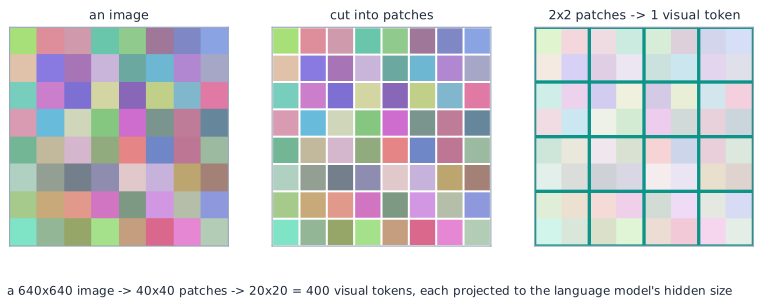
- Patchify. The image is cut into small square patches, typically 14 or 16 pixels per side. Each patch is flattened into a vector.
- Encode. A vision transformer (ViT) runs attention over all the patches at once. It’s an encoder: bidirectional, every patch sees every other patch (see the attention refresher), and there’s nothing to generate, so it’s one parallel pass.
- Project. Neighboring patch outputs are usually merged (often 2×2), and a small projector maps each merged vector to the language model’s hidden size. Each result is a visual token: it sits in the prompt exactly where an ordinary text token’s embedding would.
Counting visual tokens
With patch size and an merge, an image of pixels becomes
tokens. With 16-pixel patches merged 2×2, every 32×32-pixel area becomes one token, so a 640×640 image becomes visual tokens. Four images add 1,600 tokens to the prompt before a single word of text. Higher resolution grows the count quadratically; video multiplies it by the number of frames.
Where the cost lands
The vision encoder runs before the language model’s prefill can start, because prefill needs the visual tokens as input. So:
- The encoder adds directly to time to first token. The heavier the images, the longer the user waits.
- It’s compute-bound, like prefill: one parallel pass over many patches.
- Its output is small. It’s one vector per visual token, in the language model’s hidden size: about 7 KiB per token for a model with a 3,584-wide hidden state in BF16. Compare that with the KV cache those same tokens create once prefill processes them, which is every layer’s keys and values: several times larger.
vLLM keeps an encoder cache of these outputs, keyed by a hash of the image. A repeated image (a logo, a product photo, a diagram that appears in many prompts) can skip the encoder entirely.
The takeaway
- Images become tokens in the prompt: hundreds per image, set by resolution, patch size, and merging.
- The vision encoder is a separate model stage that runs before prefill and lands on TTFT.
- What it hands to the language model, one embedding per visual token, is small compared with the KV cache prefill builds from it.
Encoder disaggregation: splitting the vision encoder off
The guide’s first “beyond P/D” pointer is encoder disaggregation for multimodal models. Before a vision-language model can prefill a prompt containing images, every image must go through the vision encoder (the refresher above explains how). That encoder is a third phase with its own profile: a one-shot, compute-heavy pass whose cost depends on how many images arrive and at what resolution.
The problem with keeping it on the same GPU. The vLLM multimodality team’s post on encoder disaggregation (EPD) names two problems:
- Interference. A request carrying several high-resolution images occupies the GPU with encoder work, so prefill and streaming decode for everyone else become jittery, including text-only requests that never needed the encoder. It’s the long-prompt stutter from the scenario at the top, caused by pixels instead of tokens.
- Coupled scaling. Encoder, prefill, and decode all share one parallelism plan and one GPU ratio. If image traffic spikes, the only way to get more encoder capacity is to buy more full text-generation GPUs.
The design. Encoder instances run only the vision encoder; prefill/decode instances run only the language model. The request lifecycle is:
- A proxy pulls the images out of the request and sends one encoder job per image to the encoder pool.
- Encoders compute the visual-token embeddings and save them through an encoder-cache (EC) connector into shared storage, keyed by a hash of each image.
- Once every image is done, the proxy forwards the original request, now carrying only image hashes, no pixels, to a prefill/decode instance.
- That instance loads the embeddings through its own EC connector and runs prefill and decode as usual.
The EC connector mirrors the KV connector: a scheduler-side half decides what to load or save, and a worker-side half moves the data. Two benefits fall out of the design. Requests pipeline, so request 2’s images encode while request 1 is already decoding. And text-only requests skip the encoder pool entirely.
The cache is a bonus. Because embeddings land in shared storage keyed by image hash, a repeated image is encoded once and reused across users. A cached image has zero encoder cost, which comes straight off TTFT. The results below don’t separate out this effect, though.
What it bought. The team tested Qwen3-VL-4B on four A100s: one encoder instance plus three prefill/decode instances, against four data-parallel replicas of the full model. They used synthetic multimodal requests with 1–4 images of about 400 visual tokens each, and defined goodput as the highest request rate meeting a p99 TTFT of 20 s and a p99 TPOT of 100 ms:
- Short prompts (~400 text tokens): goodput barely moves with one image (23 → 24 req/s) but doubles with four (6 → 12 req/s), and p99 latencies drop 20–50%.
- Long prompts (~2,000 text tokens): the baseline sustains 4–8 req/s depending on image count; EPD sustains 8–18, 2× to 2.5× the goodput.
- Portability: the same pattern held on Ascend NPUs.
Why this cut is cheap. What crosses the encoder/prefill boundary is one embedding per visual token, in the language model’s hidden size. For a model with a 3,584-wide hidden state, that’s 7 KiB per token, compared with 56 KiB per token of KV cache at the prefill/decode boundary. Four 640×640 images come to about 11 MiB, and it crosses once per image, not once per step. Encoder disaggregation cuts the model at its narrowest waist.
My take.
- The benefit scales with how image-heavy and how mixed your traffic is. One image per request barely changed goodput; four images doubled it. Text-only traffic sharing the same GPUs is the biggest winner, and the benchmark doesn’t isolate that case.
- The SLOs are loose. A 20 s p99 TTFT is generous for interactive use. Under tighter TTFT targets, the extra proxy hop and storage round trip would matter more, and they aren’t measured separately.
- One characterization doesn’t line up. The post describes prefill as needing “high memory bandwidth” alongside large matrix multiplies, while the guide and Inside vLLM both characterize prefill as compute-bound. The roofline section above sides with the latter.
Refresher · 9 min read Mixture of experts: routing, expert parallelism, and why attention and experts behave differently What an MoE layer is, total vs active parameters, how tokens travel to experts across GPUs, and how many tokens each expert actually sees per step. Skip if You can explain top-k routing, dispatch/combine, and why an expert's efficiency depends on how many tokens reach it.
The FFN half of every layer
A transformer layer has two halves: attention, where tokens look at each other, and a feed-forward network (FFN), where each token is processed on its own by a large two-layer network. In a dense model, every token goes through the same FFN, and the FFN holds most of the model’s parameters.
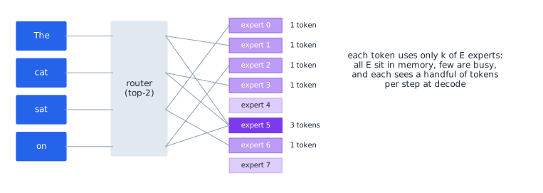
A mixture-of-experts (MoE) layer replaces that one FFN with smaller FFNs, the experts, plus a tiny router. For each token, the router scores the experts and sends the token to its top . The token’s output is the router-weighted sum of those experts’ outputs.
Total vs. active parameters
DeepSeek-V3 has 256 routed experts per MoE layer and sends each token to 8 of them. The model has 671B parameters in total, but each token only touches about 37B. That’s the appeal: the knowledge capacity of a huge model at roughly the compute cost of a much smaller one. The catch is memory. All 671B parameters must sit in GPU memory somewhere, even though any one token uses a few percent of them.
Expert parallelism: dispatch and combine
No single GPU holds all the experts of a large MoE, so they’re spread across many GPUs: expert parallelism (EP). Every MoE layer then needs two network exchanges:
- Dispatch: each GPU sends each of its tokens to the GPUs that host that token’s chosen experts.
- Combine: the expert outputs travel back and are summed.
These all-to-all exchanges happen at every MoE layer of every forward pass, so their latency sits directly on the per-token critical path. That’s why specialized communication libraries exist for this exact pattern.
How many tokens does an expert see?
Whether an expert computes efficiently depends on how many tokens reach it in one step. With tokens in a step, top- routing, and experts, the average is
An expert’s matrix multiply reads its whole weight matrix once per step, so its arithmetic intensity is roughly the number of tokens it processes (the roofline idea from the main post). In decode, each request contributes one token per step. A batch of 32 requests per GPU across 64 GPUs gives , so each of 256 experts sees tokens per step. That’s far below the few hundred needed to keep a modern GPU’s arithmetic units busy. MoE decode is memory-bound, often badly. The way out is to gather more tokens per expert: bigger batches, or more GPUs feeding the same experts.
Why attention and experts want different hardware
- Attention is stateful. It owns each request’s KV cache, which grows with the conversation; its memory needs scale with context length and the number of active requests. It also carries the request bookkeeping: scheduling and sampling.
- Experts are stateless. They hold huge, fixed weights and need many tokens per step to run efficiently, with no per-request memory at all.
Running both on the same GPUs forces one layout and one ratio on two workloads that would each prefer something different. That tension is exactly what attention–FFN disaggregation addresses.
Attention–FFN disaggregation: splitting inside every layer
The second pointer goes much deeper into the model. In a mixture-of-experts model, every layer contains two very different workloads (the MoE refresher above explains why):
- Attention is stateful. It owns the KV cache, the scheduling, and the sampling, and its needs grow with sequence length and the number of active requests.
- The experts are stateless. They hold huge weights and need many tokens per step to run efficiently, and they’re dominated by routing and all-to-all communication.
Attention–FFN disaggregation (AFD) runs them as separate services so each can be sized and laid out on its own.
The design. The vLLM AFD plugin keeps vLLM’s request path intact on the attention service: scheduler, KV cache, batching, sampling, and the OpenAI-compatible API all stay there. The FFN service is a daemon with no requests, no scheduler, and no KV cache: it receives activations plus routing metadata, computes the expert outputs, and sends them back. At every split layer, a connector ships the attention output’s hidden states to the FFN service and returns the result.
The plugin ships three connectors:
- a synchronous NCCL connector for GPUs, aimed at decode;
- a synchronous connector for Ascend NPUs, also aimed at decode;
- an asynchronous Ascend connector for prefill, which overlaps attention and expert work.
Why this cut is expensive. This is the opposite end of the spectrum from encoder disaggregation. The KV cache crosses once per request; AFD’s hidden states cross twice per MoE layer, on every forward pass, including every single decode step.
# "Both use the same idea at a different point in the model." Where you cut decides what crosses
# the wire, how big it is, and how often it must cross.
from kv_calculator import kv_bytes_per_token

KiB, MiB = 1024, 1024 ** 2

def vision_tokens(width, height, pixels_per_token=32):
    """One visual token per 32x32 pixels (16-pixel patches merged 2x2): ~400 for a 640x640 image."""
    return (width // pixels_per_token) * (height // pixels_per_token)

if __name__ == "__main__":
    # A 7B-class multimodal model: hidden size 3584, KV as in Qwen2.5-7B
    d_model, kv_tok = 3584, kv_bytes_per_token(28, 4, 128)
    n_img_tokens = 4 * vision_tokens(640, 640)
    print("Cut 1: encoder | prefill   (encoder disaggregation)")
    print(f"  crosses: one embedding per visual token = {d_model * 2 / KiB:.0f} KiB/token, once per image")
    print(f"  4 images x {vision_tokens(640, 640)} tokens -> {n_img_tokens * d_model * 2 / MiB:.1f} MiB "
          f"(the same tokens' KV cache would be {n_img_tokens * kv_tok / MiB:.0f} MiB)\n")

    print("Cut 2: prefill | decode    (P/D disaggregation)")
    print(f"  crosses: the KV cache = {kv_tok / KiB:.0f} KiB/token (Qwen2.5-7B), once per request\n")

    # DeepSeek-V3: hidden 7168, 61 layers (58 MoE), MLA caches 512 + 64 values per token per layer
    ds_d, ds_moe_layers, ds_layers = 7168, 58, 61
    ds_kv = (512 + 64) * ds_layers * 2
    af = 2 * ds_d * 2 * ds_moe_layers                      # hidden state out and FFN output back, bf16
    print("Cut 3: attention | FFN     (attention-FFN disaggregation, MoE)")
    print(f"  crosses: hidden states out and back at every MoE layer = {af / MiB:.2f} MiB per token per forward pass")
    print(f"  DeepSeek-V3's whole KV cache is {ds_kv / KiB:.0f} KiB per token, sent once;"
          f" the A|F cut moves {af / ds_kv:.0f}x that, on EVERY decode step\n")

    # MoE: how many tokens does each expert see per step?
    experts, top_k = 256, 8
    print("Why the attention:FFN ratio matters (DeepSeek-V3 routing: 256 experts, top-8)")
    for attn_ranks in (48, 64):
        for batch in (32, 128):
            per_expert = attn_ranks * batch * top_k / experts
            print(f"  {attn_ranks} attention ranks x {batch:3d} decode tokens each -> {per_expert:5.0f} tokens per expert per step")
    print("  (an expert's matmul has arithmetic intensity of roughly its token count; the GPU ridge is a few hundred)\n")

    # Hybrid SSM: a Mamba layer's state is a fixed-size summary, unlike per-token KV
    ssm_state = 48 * 64 * 128 * 4 + 3 * 3072 * 2           # SSM state (fp32) + conv state (bf16), per GPU at TP=2
    fa_per_token_layer = 2 * 4 * 128 * 2                    # one attention layer's KV per token, same model
    print("Hybrid SSM (Nemotron-3-Nano example, per GPU at TP=2, per layer, per request)")
    print(f"  Mamba state: {ssm_state / MiB:.2f} MiB, fixed;  attention KV: {fa_per_token_layer / KiB:.0f} KiB per token")
    print(f"  break-even: a Mamba layer's state is smaller than an attention layer's KV beyond "
          f"{ssm_state / fa_per_token_layer:,.0f} prompt tokens")
Cut 1: encoder | prefill (encoder disaggregation)
crosses: one embedding per visual token = 7 KiB/token, once per image
4 images x 400 tokens -> 10.9 MiB (the same tokens' KV cache would be 88 MiB)
Cut 2: prefill | decode (P/D disaggregation)
crosses: the KV cache = 56 KiB/token (Qwen2.5-7B), once per request
Cut 3: attention | FFN (attention-FFN disaggregation, MoE)
crosses: hidden states out and back at every MoE layer = 1.59 MiB per token per forward pass
DeepSeek-V3's whole KV cache is 69 KiB per token, sent once; the A|F cut moves 24x that, on EVERY decode step
Why the attention:FFN ratio matters (DeepSeek-V3 routing: 256 experts, top-8)
48 attention ranks x 32 decode tokens each -> 48 tokens per expert per step
48 attention ranks x 128 decode tokens each -> 192 tokens per expert per step
64 attention ranks x 32 decode tokens each -> 64 tokens per expert per step
64 attention ranks x 128 decode tokens each -> 256 tokens per expert per step
(an expert's matmul has arithmetic intensity of roughly its token count; the GPU ridge is a few hundred)
Hybrid SSM (Nemotron-3-Nano example, per GPU at TP=2, per layer, per request)
Mamba state: 1.52 MiB, fixed; attention KV: 2 KiB per token
break-even: a Mamba layer's state is smaller than an attention layer's KV beyond 777 prompt tokensFor a DeepSeek-V3-family model, AFD moves about 1.6 MiB per token per forward pass: 24 times the model’s entire per-token KV cache, on every step. That traffic is latency-critical, sitting directly between attention and the next layer. It only pays off with very fast interconnects and with communication overlapped against computation, which is why the plugin supports dual-batch overlap.
What it bought. The plugin’s published decode benchmark compares a conventional 64-way expert-parallel deployment with two AFD layouts on Ascend 910C, for DeepSeek-V3.2. Output is normalized per chip:
- 48 attention + 16 FFN chips: 5–10% slower than the baseline.
- 64 attention + 16 FFN chips: 9–11% faster (258.9 vs 232.6 tokens/s per chip at 16K input).
The authors draw the right lesson: the attention-to-FFN ratio matters, and disaggregation alone doesn’t guarantee a gain. The token-per-expert numbers above show why. More attention ranks feeding the same experts means more tokens per expert per step, and decode experts are starved for tokens. The authors note the FFN ranks still had headroom at the ratios they tried. An early prefill experiment cut median TTFT from 15.1 s to 8.0 s at 12 req/s.
My take: promising, and explicitly early. Read the fine print before quoting those numbers:
- The routing was forced. Expert routing was replaced by a deterministic balancing pattern, which changes the model’s outputs. Real routing is uneven, and unevenness is precisely what makes MoE serving hard.
- The scale was simulated. The physical deployments stood in for logical ones four times larger.
- The prefill test used a 10-layer slice of the model.
- Narrow support. The plugin is pinned to one vLLM version and keeps full weights on both roles.
The ratio insight is the durable lesson. The specific percentages aren’t, yet.
Hybrid SSM models: transferring a state, not a cache
The last pointer extends ordinary P/D to hybrid models that interleave attention layers with Mamba-style state-space (SSM) layers, such as NVIDIA’s Nemotron-H family. The complication is that the two layer types remember the past in completely different shapes:
- An attention layer stores per-token keys and values, which grow with the prompt.
- A Mamba layer stores a fixed-size state: a small convolution buffer plus a recurrent state that summarizes the entire history, regardless of length. There are no “tokens” in it to page or slice.
The cut-points program above puts numbers on it. In the Red Hat and vLLM post’s example model, one Mamba layer’s state is about 1.5 MiB per request, while one attention layer’s KV is 2 KiB per token, so beyond roughly 780 prompt tokens the Mamba layer is the cheaper one to ship, and it stays constant however long the conversation gets.
The Red Hat and vLLM team behind this support extended the NIXL connector to describe the same GPU memory two ways at once, as attention blocks and as Mamba state blocks. That lets one RDMA read move both. They also reorganized the convolution state so that decode GPUs with a different tensor-parallel layout can each read exactly their own slice, with no staging buffers and no reshuffling. On eight H200s serving a 120B hybrid MoE, disaggregated P/D beat a single 8-GPU instance at high concurrency, the same pattern as for ordinary transformers.
One echo of my CLM review: there, Suffix Cache Reuse had to resume linear-attention layers from a saved state snapshot, because you can’t remove a token from the middle of a recurrent state. The same property shapes this design: an SSM state can only be handed over whole, as of a point in the sequence.
Same idea, different cut
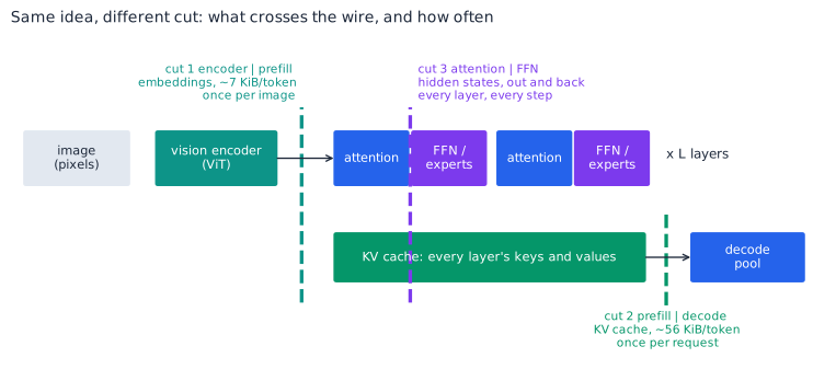
Put side by side, the guide’s sentence that these designs share “the same idea at a different point in the model” becomes a single trade-off. Every disaggregation isolates two kinds of work that interfere, and pays for it with whatever must cross the cut:
| Cut | What crosses | Size (per token) | How often | Worth it when |
|---|---|---|---|---|
| Encoder / prefill | Visual embeddings | ~7 KiB | Once per image | Image-heavy or mixed traffic |
| Prefill / decode | KV cache (or SSM state) | ~56–320 KiB | Once per request | Long prompts, tight ITL targets, fast links |
| Attention / FFN | Hidden states, both ways | ~1.6 MiB per pass | Every layer, every step | Large MoE, very fast interconnect, overlap |
The further into the model you cut, the more often you pay, and the more the interconnect has to be part of the design rather than an afterthought.
What it buys you, and what it costs
Refresher · 6 min read Tensor, pipeline, data, and expert parallelism in one page The four ways to spread a model across GPUs, what each one splits, what it costs in communication, and what it's good for in serving. Skip if You know what TP=8 means, why it needs fast links, and how it differs from running replicas.
Four ways to use more than one GPU
- Tensor parallelism (TP) splits every layer’s matrices across GPUs. Each GPU holds a slice of every weight matrix and computes its slice of every matrix multiply, then the GPUs combine partial results with an all-reduce, typically twice per layer. TP makes one request faster and lets a model larger than one GPU fit. The price is constant communication, so it wants very fast links (NVLink) and usually stays inside one server.
- Pipeline parallelism (PP) splits the model by layers: GPU 1 runs layers 1–20, GPU 2 runs layers 21–40, and so on. It communicates less than TP (only activations between stages), but a single request has to pass through the stages one after another.
- Data parallelism (DP) runs independent full copies of the model, called replicas, and spreads requests across them. It adds capacity, not speed for any single request, and needs almost no communication.
- Expert parallelism (EP) spreads a mixture-of-experts model’s experts across GPUs and routes each token to the GPUs holding its chosen experts (see the MoE refresher).
These combine. “TP=4, DP=2” on eight GPUs means two replicas, each split four ways.
Why the phases want different choices
Prefill is compute-bound, so splitting its matrix multiplies across more GPUs cuts the time to first token almost proportionally. The all-reduces carry large messages (one hidden vector per prompt token) but usually overlap well with the heavy computation.
Decode is memory-bound, and its sizing question is different: how many streams can run at once while every step stays under the inter-token latency target? That’s limited by KV-cache memory (whatever’s left after the weights) and by the per-step time. Decode’s all-reduces are tiny, so their fixed latency, not their bandwidth, is what costs.
A shared deployment has to use one layout for both phases. Separate pools can choose independently.
Two knobs instead of one
The guide’s first benefit is that TTFT and ITL can be tuned independently: each tier gets the parallelism that suits its own phase. Prefill can be tensor-parallel-heavy and decode can be sized for batch, and changing one doesn’t drag the other with it.
In a shared deployment, there’s one layout and one set of knobs. Give the instance more GPUs per replica to cut TTFT, and you’ve also changed how many decode streams fit, how big each decode step is, and how much memory is left for KV cache. Every change moves both numbers at once.
With separate pools, each one answers its own question. The parallelism refresher above explains the terms; here are the two questions for Llama-3.1-70B on H100s, with the assumptions written into the code:
# "Prefill can be TP-heavy, decode can be sized for batch." Two pools, two different questions.
# Llama-3.1-70B on H100 SXM (BF16). Illustrative assumptions, stated up front:
PARAMS, LAYERS, D_MODEL = 70.6e9, 80, 8192
KV_TOKEN = 327_680                        # bytes per token (80 layers x 8 KV heads x 128 x 2 x 2)
HBM, BW, FLOPS = 80e9, 3.35e12, 989e12    # per GPU: memory, bandwidth, dense BF16 peak
ETA_C, ETA_B = 0.45, 0.75                 # achieved fraction of peak compute / bandwidth
NVLINK = 450e9                            # bytes/s per direction per GPU
AR_LATENCY = 15e-6                        # fixed cost of one small all-reduce (decode)
WEIGHTS = PARAMS * 2

def prefill_ttft(tokens, tp):
    """Compute-bound: more GPUs per instance -> shorter prefill, minus all-reduce traffic."""
    compute = 2 * PARAMS * tokens / (tp * FLOPS * ETA_C)
    allreduce = 2 * LAYERS * 2 * (tp - 1) / tp * tokens * D_MODEL * 2 / NVLINK   # 2 all-reduces per layer
    return compute + allreduce

def decode(tp, context=4096, itl_slo=0.040, mem_util=0.9):
    """Memory-bound: the batch is capped by KV memory and by the ITL target."""
    kv_room = tp * HBM * mem_util - WEIGHTS
    max_batch_mem = int(kv_room // (KV_TOKEN * context))
    base = WEIGHTS / tp / (BW * ETA_B) + 2 * LAYERS * AR_LATENCY
    per_stream = KV_TOKEN * context / tp / (BW * ETA_B)
    max_batch_slo = int((itl_slo - base) / per_stream)
    b = min(max_batch_mem, max_batch_slo)
    itl = base + b * per_stream
    return b, itl, b / itl / tp, "memory" if max_batch_mem < max_batch_slo else "ITL target"

if __name__ == "__main__":
    print("Prefill pool: time to first token for one 8,192-token prompt")
    for tp in (4, 8):
        print(f"  TP={tp}: {prefill_ttft(8192, tp) * 1e3:5.0f} ms")
    print("\nDecode pool: largest batch per instance at 4K context with ITL <= 40 ms")
    print(f"  {'layout':10s} {'batch':>6s} {'ITL':>8s} {'tokens/s per GPU':>17s}  limited by")
    for tp in (4, 8):
        b, itl, tput, limit = decode(tp)
        print(f"  TP={tp:<7d} {b:6d} {itl * 1e3:6.1f} ms {tput:15,.0f}    {limit}")
Prefill pool: time to first token for one 8,192-token prompt
TP=4: 721 ms
TP=8: 408 ms
Decode pool: largest batch per instance at 4K context with ITL <= 40 ms
layout batch ITL tokens/s per GPU limited by
TP=4 109 31.0 ms 879 memory
TP=8 323 31.0 ms 1,303 memory- The prefill pool asks: how many GPUs should work on one prompt? It’s compute-bound, so going from 4-way to 8-way tensor parallelism cuts an 8K-token TTFT from about 720 to about 410 ms, even after paying for the all-reduces.
- The decode pool asks: how many streams fit under the ITL target? Here both layouts are limited by memory, not speed. Each replica must hold a full copy of the 141 GB of weights, so an 8-way instance leaves far more room for KV cache than a 4-way one, fits three times the streams, and delivers about 50% more tokens per GPU at the same 31 ms ITL.
The two pools might land on the same layout or on different ones. The point is that each decision is made against its own target, with no compromise between them.
Flat tails, and why chunking only gets you partway
The second benefit is about tails: a decode instance that only ever runs decode batches never has a long prefill stall its streams. The guide adds that chunked prefill gets you partway there, but the right chunk size depends on the traffic, so you end up retuning it.
The simulator shows why “retuning” is the right word. Here’s the collocated server from the benchmark, with the prefill chunk size swept at two loads:
# "The right chunk size depends on the traffic, so you end up retuning it."
# Collocated serving, same benchmark as before, sweeping the prefill token budget per step.
import numpy as np
from serving_sim import run, run_requests

BUDGETS = [512, 1024, 2048, 4096, 8192]
if __name__ == "__main__":
    for rate in (0.4, 1.0):
        print(f"offered load {rate} req/s")
        print(f"  {'tokens/step':>11s} {'median TTFT':>12s} {'p99 ITL':>9s} {'worst gap':>10s}")
        for b in BUDGETS:
            ttft, _, p99 = np.array([run(rate, "collocated", 0, seed=s, budget=b) for s in range(5)]).mean(axis=0)
            worst = np.mean([run_requests(rate, "collocated", 0, seed=s, budget=b)[:, 2].max() for s in range(5)])
            print(f"  {b:11,d} {ttft:10.2f} s {p99 * 1e3:7.0f} ms {worst * 1e3:8.0f} ms")
offered load 0.4 req/s
tokens/step median TTFT p99 ITL worst gap
512 0.77 s 49 ms 51 ms
1,024 0.76 s 94 ms 99 ms
2,048 0.75 s 174 ms 194 ms
4,096 0.74 s 89 ms 376 ms
8,192 0.74 s 28 ms 710 ms
offered load 1.0 req/s
tokens/step median TTFT p99 ITL worst gap
512 0.78 s 51 ms 51 ms
1,024 0.77 s 99 ms 99 ms
2,048 0.76 s 194 ms 194 ms
4,096 0.75 s 376 ms 376 ms
8,192 0.75 s 710 ms 710 ms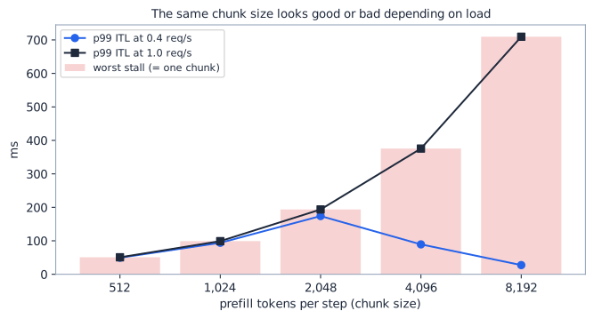
Two things happen at once:
- The worst stall is exactly one chunk, whatever the load: about 50 ms at 512 tokens, 710 ms with no chunking at all.
- The p99 depends on how often chunks happen to collide with streams, so it moves with load. At 0.4 req/s, no chunking has the best p99 of all (28 ms): its 710 ms stalls are rare enough to hide below the 99th percentile. At 1.0 req/s, the same setting has the worst p99 (710 ms).
A chunk size tuned on last month’s traffic can be wrong for this month’s. Smaller chunks also have a cost my model understates: GPUs run small matrix multiplies less efficiently, so very small chunks stretch the newcomer’s TTFT. Disaggregation removes the knob altogether, which is why vLLM’s own docs call it the more reliable way to control tail ITL.
“Every first token pays for the transfer”
This short sentence is the whole cost side of P/D. In a collocated server, a request’s first token comes straight out of its prefill. In disaggregated serving, the path is longer:
- The prefill instance computes the prompt’s KV cache, generating a single token (the proxy asks it for at most one).
- It holds the blocks and replies to the proxy.
- The proxy sends the request on to a decode instance, along with the location of those blocks.
- Decode pulls the blocks across.
- Decode notices the transfer has finished, at its next step boundary.
- Decode runs its first step, which produces the token the user actually sees.
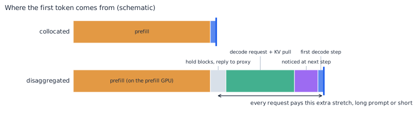
In symbols:
- : queueing and prefill on the prefill pool, the same as collocated minus the interference.
- : the new cost, made of the KV transfer, the notification, and the proxy hops.
- : the first decode step.
“Every” is the key word. The handoff applies to every request, including short prompts that never caused any interference in the first place. P/D only wins on TTFT when the queueing and interference it removes outweigh the handoff it adds. On the guide’s test box, the handoff was 1.3 s, mostly overhead rather than bandwidth, and that alone pushed every first token past a 2 s target. With layer-by-layer streaming over a fast link (the KV section above; fabric-lib does this, vLLM’s NIXL connector does not yet), the same handoff shrinks to milliseconds.
“The CPU tier is cheap”
The guide’s argument has three parts:
- Once templating, tokenization, and parsing move off the GPU box, they scale with CPU load instead of consuming accelerator time.
- The render tier does real work in three places: long prompts, multimodal preprocessing, and reasoning or tool parsing. None of it needs a GPU.
- The concrete number: templating and tokenizing a 9,000-token chat prompt for Qwen2.5-7B took about 15 ms of CPU.
Let’s put numbers on all of it:
# "The CPU tier is cheap." How much CPU does rendering take, and where does it get heavy?
import io, time
import numpy as np
from PIL import Image

# 1. Text: the guide measured ~15 ms of CPU to template + tokenize a 9,000-token chat prompt.
US_PER_TOKEN = 15e-3 / 9000 * 1e6
print(f"1. Text rendering: ~{US_PER_TOKEN:.1f} microseconds of CPU per prompt token (from the guide's measurement)")
print(f"   {'prompt tokens':>13s} {'req/s':>6s} {'CPU cores busy':>15s}")
for tokens, rate in [(9000, 0.4), (9000, 73), (2000, 500), (100_000, 20)]:
    cores = rate * tokens * US_PER_TOKEN * 1e-6
    print(f"   {tokens:13,d} {rate:6g} {cores:15.2f}")

# 2. Images: decode a JPEG, resize, normalize -- measured here, on this machine's CPU.
rng = np.random.default_rng(0)
photo = Image.fromarray(rng.integers(0, 255, (1080, 1920, 3), dtype=np.uint8))
buf = io.BytesIO(); photo.save(buf, format="JPEG", quality=90); jpeg = buf.getvalue()
def preprocess(data):
    img = Image.open(io.BytesIO(data)).convert("RGB").resize((640, 640), Image.BICUBIC)
    x = np.asarray(img, dtype=np.float32) / 255.0
    return (x - x.mean(axis=(0, 1))) / (x.std(axis=(0, 1)) + 1e-6)
preprocess(jpeg)
t = time.perf_counter(); runs = 20
for _ in range(runs): preprocess(jpeg)
ms = (time.perf_counter() - t) / runs * 1e3
print(f"\n2. Image preprocessing (1080p JPEG -> 640x640 normalized), measured: {ms:.1f} ms of CPU per image")
print(f"   a request with 4 images: ~{4 * ms:.0f} ms of CPU before the vision encoder can start")

# 3. Streaming through a reasoning/tool parser on a stateless render tier: replay cost grows ~ n^3.
print("\n3. Streaming parser replay (see the earlier program): doubling the output multiplies the work by ~8")
1. Text rendering: ~1.7 microseconds of CPU per prompt token (from the guide's measurement)
prompt tokens req/s CPU cores busy
9,000 0.4 0.01
9,000 73 1.09
2,000 500 1.67
100,000 20 3.33
2. Image preprocessing (1080p JPEG -> 640x640 normalized), measured: 70.7 ms of CPU per image
a request with 4 images: ~283 ms of CPU before the vision encoder can start
3. Streaming parser replay (see the earlier program): doubling the output multiplies the work by ~8Read it as three cases:
- Text is cheap, and it scales linearly. The guide’s 15 ms for 9,000 tokens works out to about 1.7 µs of CPU per token. At the guide’s low benchmark load that’s 1% of one core; at 73 requests per second it’s about one core, which matches the guide’s measured ceiling for one render server. A 100K-token agent context at 20 req/s keeps more than three cores busy just tokenizing.
- Images are where the CPU tier earns its name. Decoding, resizing, and normalizing one 1080p JPEG took about 70 ms of CPU on the machine I ran this on. That’s a pessimistic figure, since my test image is random noise, which compresses badly and decodes slowly. Still, a four-image request can need a quarter-second of preprocessing before the vision encoder even starts. On a GPU box, that work competes for the same CPU cores that feed the GPUs.
- Streaming parsers are the expensive case, as the earlier program showed: on a stateless tier, the work grows with the cube of the output length.
Why does it matter that this runs off the GPU box, if it’s cheap? Two reasons:
- Cost. A GPU server is priced for its accelerators; its CPU cores are a small part of the bill, and you can’t buy more of them without buying more GPUs. A separate CPU tier scales on cheap cores, independently.
- Interference. The serving engine’s own scheduling loop runs on the CPU. Heavy preprocessing or parsing on the same cores can delay the next GPU step, a smaller cousin of the prefill stall. A tier you can scale on its own, with no per-request state, is the cleanest fix.
Expert recommendations: when to split, and when not to
The guide ends its cost-benefit section with a decision table matching situations to recommendations; the right-hand pane opens it at the table. Here is the same advice as a decision flow, with two additions from this review: check the handoff before anything else, and guard multi-turn reuse when the conversation history can change.
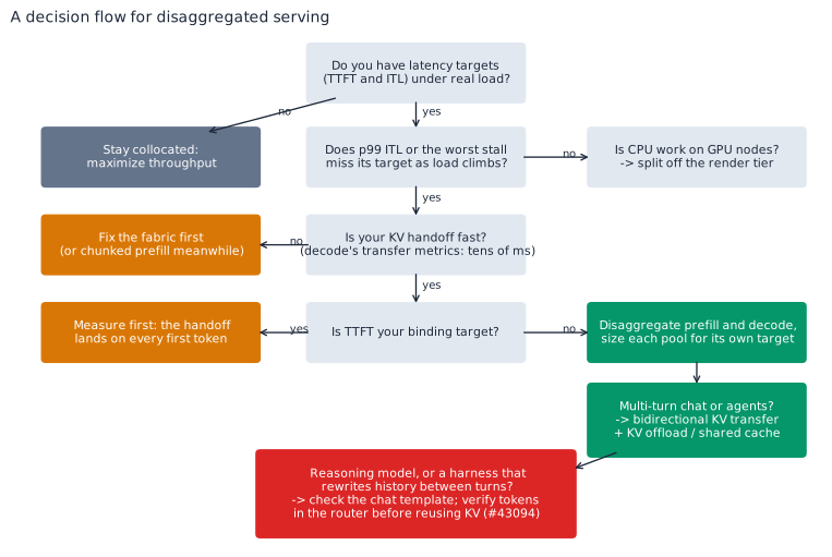
In prose:
- No latency targets, or low, bursty traffic? Stay collocated and maximize throughput; disaggregation doesn’t raise it.
- Tail ITL missing its target under real load is the main reason to disaggregate, and long prompts at high concurrency are where it bites hardest.
- But only if the KV handoff is fast. Check decode’s transfer metrics first. A slow handoff lands on every first token and caps throughput, so fix the fabric, or stay collocated meanwhile.
- If TTFT is your binding target, measure before you split, for the same reason.
- If CPU work shows up on your GPU nodes, split off the render tier. That’s independent of everything above.
- For multi-turn chat and agents, disaggregate with bidirectional transfer, and pair it with KV offloading or a shared KV cache.
- For reasoning models, or any harness that rewrites history between turns, check the chat template and verify tokens before reusing KV (see the reasoning-model warning below).
Running P/D: let decode reuse prefill’s token IDs
The guide’s “easy win” makes sense once you see what the proxy does. For each request, it sends the same chat request, the list of messages, first to prefill and then to decode. Both are ordinary chat-completions endpoints, so by default both render the chat template and tokenize the result. That’s the 15 ms of CPU per 9,000-token prompt from above, done twice.
The fix is two fields:
- Ask prefill to return the token IDs it produced (
return_token_ids). - Have the proxy hand them to decode inside
kv_transfer_params(asprompt_token_ids).
Decode then skips templating and tokenization entirely. It still needs the messages, because its parsers use them to split reasoning, content, and tool calls. vLLM’s latest docs add two conditions (not yet in the v0.30.0 release): if the messages contain non-text content (images, say) or the request uses echo, decode ignores the IDs and renders the messages itself, and malformed IDs fail the request with a 400.
There’s a quieter benefit too. Rendering twice means trusting that both renders agree, and chat templates aren’t always deterministic. Some stamp the current date into the system prompt:
# "The prefill stage already tokenized the prompt." In P/D over /v1/chat/completions, the proxy sends
# the SAME chat request (messages) to prefill and then to decode, so by default BOTH render the chat
# template and tokenize it. Reusing prefill's token IDs saves decode that CPU work -- and guarantees
# decode holds exactly the token IDs whose KV cache it just received.
from datetime import datetime
from jinja2 import Template
from render_derender_toy import tokenize

# Some chat templates stamp the current date into the system prompt.
TEMPLATE = Template("<|start|>system\nToday is {{ today }}.<|end|>\n"
                    "{% for m in messages %}<|start|>{{ m.role }}\n{{ m.content }}<|end|>\n{% endfor %}"
                    "<|start|>assistant\n")

def render(messages, now):
    return tokenize(TEMPLATE.render(messages=messages, today=now.strftime("%d %b %Y")))

messages = [{"role": "user", "content": "Weather in Paris?"}]

# Default P/D flow: each stage renders and tokenizes on its own, a moment apart.
prefill_ids = render(messages, datetime(2026, 10, 3, 23, 59, 59, 900_000))   # prefill runs just before midnight
decode_ids = render(messages, datetime(2026, 10, 4, 0, 0, 0, 300_000))       # decode renders 0.4 s later
diff = [i for i, (a, b) in enumerate(zip(prefill_ids, decode_ids)) if a != b]
print(f"prefill tokenized {len(prefill_ids)} tokens; decode re-tokenized {len(decode_ids)} tokens")
print(f"they differ at positions {diff}: decode would hold KV computed for different tokens than its own prompt")

# The easy win: prefill returns its token IDs (return_token_ids), and the proxy hands them to decode
# inside kv_transfer_params["prompt_token_ids"]. Decode skips templating and tokenization entirely.
kv_transfer_params = {"do_remote_prefill": True, "prompt_token_ids": prefill_ids}
print(f"\nwith reuse: decode uses prefill's {len(kv_transfer_params['prompt_token_ids'])} IDs, one tokenization, one truth")
print(f"CPU saved per request: about {9000 * 15 / 9000:.0f} ms for a 9,000-token prompt (the guide's measurement)")
prefill tokenized 42 tokens; decode re-tokenized 42 tokens
they differ at positions [18]: decode would hold KV computed for different tokens than its own prompt
with reuse: decode uses prefill's 42 IDs, one tokenization, one truth
CPU saved per request: about 15 ms for a 9,000-token prompt (the guide's measurement)A request that straddles midnight renders two different prompts: prefill computed KV for one, while decode holds token IDs for the other. It’s an edge case, but vLLM won’t catch it: decode sizes the KV transfer from its own prompt and pairs blocks with prefill’s by position, never comparing tokens, so a same-length mismatch like this one silently attends to keys and values computed for prefill’s tokens. But it shows the principle behind the easy win: one tokenization means one truth about what the KV cache describes.
Refresher · 6 min read Multi-turn conversations and KV reuse Why every chat turn resends the whole conversation, how a single server avoids recomputing it, and what changes when prefill and decode are separate machines. Skip if You know which tokens a prefix cache can and can't reuse on turn two of a conversation.
Every turn resends everything
Chat APIs are stateless: on turn two, the client sends the system prompt, the first user message, the model’s first answer, and the new message, all of it, again (see the agent-loop refresher). Agents make this extreme. A coding agent can run dozens of turns per session, each one replaying a context that only grows.
A single server reuses almost all of it
On one vLLM engine, the KV cache for turn one’s prompt and for the answer it generated sit in the same paged memory. With prefix caching on, turn two’s prompt matches all of those blocks by hash (see the KV-caching refresher), so the engine computes only the new message. Time to first token on turn five can be a fraction of turn one’s.
Disaggregation splits the history across two machines
With separate prefill and decode instances, the history is split:
- Prefill computed turn one’s prompt, so it can cache those blocks.
- Decode generated the answer, so only decode has the answer’s KV.
On turn two, prefill sees a prompt containing an answer it never computed. In standard, one-way P/D, it recomputes that answer, every turn. The longer the model’s answers (reasoning traces, tool calls), the more work that is.
Bidirectional KV transfer closes the loop. Decode keeps its blocks for a while after the turn, and on the next turn prefill pulls the blocks it’s missing back from decode, then computes only the new message. Something has to remember which blocks belong to which conversation; in vLLM, that’s a proxy keyed by a conversation ID the client sends.
The assumption underneath
Every form of KV reuse assumes the new prompt continues the old sequence: same tokens, same positions, with new tokens only at the end. A single server’s prefix cache checks that assumption block by block, so a mismatch only costs a recompute. Any mechanism that reuses blocks without checking turns a broken assumption into wrong output.
Multi-turn: stop recomputing the conversation
Standard P/D moves the cache one way, which the guide calls wasteful for chat and agent loops (the refresher above sets up why). On turn two, decode still holds KV for the answer it just generated, but prefill never computed that answer, so prefill recomputes it. With bidirectional_kv_xfer set on both instances, prefill pulls those blocks back from decode instead and computes only the new tokens.
A proxy tracks which blocks belong to which conversation, keyed by a conversation_id the client sends with each request. vLLM’s NixlConnector docs add the two settings that matter: bidirectional transfer is off by default, and decode keeps a conversation’s blocks for 480 seconds by default (decoder_kv_blocks_ttl) waiting for the next turn.
Here’s what each design computes on every turn of a six-turn conversation:
# Multi-turn chat under three designs. Each turn resends the whole conversation; what matters is how
# much of it the prefill engine must actually compute. Qwen2.5-7B on an L40S, as in the guide's benchmark.
from roofline import prefill
from serving_sim import step_time
from kv_calculator import kv_bytes_per_token

FIRST_PROMPT, ANSWER, NEW_MSG, TURNS = 4000, 600, 400, 6
KV = kv_bytes_per_token(28, 4, 128)

def ttft_ms(new_tokens, cached):
    return step_time(*prefill(new_tokens, past=cached)) * 1e3

print(f"first prompt {FIRST_PROMPT} tokens; each answer {ANSWER}; each follow-up message {NEW_MSG}\n")
print(f"{'turn':>4s} {'history':>8s} | {'collocated + prefix cache':>26s} | {'P/D one-way':>18s} | {'P/D bidirectional':>30s}")
history = 0
for turn in range(1, TURNS + 1):
    new = FIRST_PROMPT if turn == 1 else NEW_MSG
    # Collocated: the same engine generated the last answer, so its KV is already cached.
    c = ttft_ms(new, history)
    # One-way P/D: prefill never saw the last answer (decode generated it), so it recomputes it.
    redo = 0 if turn == 1 else ANSWER
    o = ttft_ms(new + redo, history - redo)
    # Bidirectional: prefill pulls back the blocks it lacks (decode's last answer) and computes only the
    # new tokens; earlier turns are assumed still in prefill's own prefix cache.
    pulled = 0 if turn == 1 else ANSWER
    b = ttft_ms(new, history)
    print(f"{turn:4d} {history:8,d} | {new:>6,d} new -> {c:5.0f} ms     | {new + redo:>5,d} -> {o:5.0f} ms | "
          f"{new:>5,d} -> {b:5.0f} ms + pull {pulled * KV / 2**20:3.0f} MiB")
    history += new + ANSWER
first prompt 4000 tokens; each answer 600; each follow-up message 400
turn history | collocated + prefix cache | P/D one-way | P/D bidirectional
1 0 | 4,000 new -> 328 ms | 4,000 -> 328 ms | 4,000 -> 328 ms + pull 0 MiB
2 4,600 | 400 new -> 37 ms | 1,000 -> 89 ms | 400 -> 37 ms + pull 33 MiB
3 5,600 | 400 new -> 38 ms | 1,000 -> 92 ms | 400 -> 38 ms + pull 33 MiB
4 6,600 | 400 new -> 39 ms | 1,000 -> 94 ms | 400 -> 39 ms + pull 33 MiB
5 7,600 | 400 new -> 40 ms | 1,000 -> 96 ms | 400 -> 40 ms + pull 33 MiB
6 8,600 | 400 new -> 41 ms | 1,000 -> 99 ms | 400 -> 41 ms + pull 33 MiB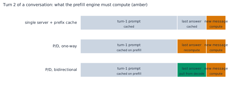
After the first turn, a single server with prefix caching computes only the new message: about 40 ms here. One-way P/D recomputes the previous answer on top, roughly 2.4 times the work, on every turn. Bidirectional transfer brings P/D back to the single-server cost, plus a 33 MiB pull of the last answer’s blocks. That’s why the guide’s advice is to measure TTFT on turn five, not turn one: the first turn looks the same everywhere.
The longer the model’s answers, the bigger the gap. Agents, with long tool calls and long reasoning, are the extreme case: vLLM’s analysis of agentic traffic reports a median of 43 turns per session.
One housekeeping note: the guide links a dedicated post on bidirectional KV transfer, but that link returned a 404 when I checked. The NixlConnector documentation covers the feature in the meantime.
Refresher · 7 min read Reasoning models: thinking tokens, parsers, and what the next turn sees What makes a model a 'reasoning' model, how its thinking is separated from its answer, and why chat templates often drop old thinking from the conversation. Skip if You know what a <think> block is, what a reasoning parser does, and whether your model's chat template keeps or strips past reasoning.
Thinking before answering
A reasoning model (DeepSeek-R1, Qwen3 in thinking mode, and many others) is trained to generate an explicit chain of thought before its answer. Reinforcement learning with outcome rewards, such as GRPO (see the policy-gradients and DeepSeekMath refreshers), taught these models that writing out intermediate steps leads to more correct answers. The thinking is just more generated tokens, wrapped in delimiters, often <think> and </think>:
<think>The user wants 17 x 23. 17 x 20 = 340, 17 x 3 = 51, total 391.</think>
17 x 23 = 391.
Thinking traces are often long, hundreds to thousands of tokens, which is why reasoning models are expensive to serve: every thinking token is a decode step.
Separating thinking from answer
The model produces one stream of tokens; the API returns structured fields. A reasoning parser on the server finds the delimiters and splits the output into reasoning and content (this is part of the “third job” CPU work). Streaming makes the parser stateful: it has to track whether it’s currently inside a thinking block as chunks arrive.
What happens to old thinking on the next turn?
When the client sends turn two, the conversation history contains turn one’s assistant message. The model’s chat template decides how that message is turned back into tokens, and many templates drop the thinking from past assistant turns, keeping only the final answer. Qwen3’s template does this on its own. The reasons are practical:
- Context budget. Old reasoning is long, and it’s rarely needed once the answer exists.
- Training match. Models were trained on conversations formatted that way.
Some models and agent setups deliberately keep reasoning across turns instead, for example so an agent can keep its plan between tool calls; vLLM documents this under interleaved thinking.
Why it matters for serving
Stripping old thinking means the next prompt is not a continuation of what the model generated: tokens disappear from the middle of the sequence. Anything that reused KV computed for the original sequence now faces a sequence with a hole in it. For a prefix cache that checks block contents, that’s a cache miss after the hole. For anything that reuses blocks by position, it’s a correctness problem, which is the warning in the main post.
The reasoning-model warning: wrong, not slow
The guide’s warning, in plain terms:
- What decode holds. On a reasoning model, decode’s blocks cover everything it generated, including the thinking.
- What comes back. Many chat templates drop old thinking when the next turn is rendered; Qwen3’s does so automatically. The next prompt is then the old prompt, the visible answer, and the new message, with the thinking missing from the middle.
- What breaks. Prefill’s prompt no longer lines up with decode’s blocks, and the result is wrong output, not just slow output.
- No safety net. Nothing in vLLM catches the mismatch today, so check your chat template before turning bidirectional transfer on.
The GitHub issue the guide cites explains the mechanism. When prefill pulls blocks back from decode, the selection is positional: it takes the last blocks of decode’s sequence, assuming prefill’s prompt is a strict prefix of what decode generated. With the thinking stripped out, that assumption is false, and prefill loads KV computed for different tokens at different positions. Here’s the failure reconstructed at toy scale:
# Why stripped thinking traces make bidirectional KV transfer WRONG, not just slow.
# Reconstructed from vLLM issue #43094 with tiny sizes: block size 4, one-letter "tokens".
import hashlib

BLOCK = 4
prompt   = [f"p{i}" for i in range(8)]       # turn-1 prompt (prefill has these blocks cached locally)
thinking = [f"t{i}" for i in range(6)]       # the reasoning trace decode generated
answer   = [f"a{i}" for i in range(6)]       # the visible answer decode generated
new_msg  = [f"u{i}" for i in range(4)]       # the user's next message

decode_seq = prompt + thinking + answer                  # what decode's KV blocks actually cover
turn2      = prompt + answer + new_msg                   # what the chat template sends: thinking stripped

def blocks(seq):
    return [seq[i:i + BLOCK] for i in range(0, len(seq) - len(seq) % BLOCK, BLOCK)]

local_cached = len(blocks(prompt))                       # prefill already holds the prompt's blocks
needed = len(blocks(prompt + answer)) - local_cached     # full blocks prefill lacks before the new message
print(f"decode's blocks: {blocks(decode_seq)}")
print(f"turn-2 prompt  : {turn2}\n")

# The positional shortcut: assume prefill's prompt is a prefix of decode's sequence and take the
# LAST `needed` blocks from decode (the suffix-trimming step described in the issue).
pulled = blocks(decode_seq)[-needed:]
start = local_cached * BLOCK
expected = [turn2[start + i * BLOCK:start + (i + 1) * BLOCK] for i in range(needed)]
for got, want in zip(pulled, expected):
    print(f"positions {start}-{start + BLOCK - 1}: prefill needs KV for {want}")
    print(f"                 but loads decode's KV for {got}, computed at positions "
          f"{decode_seq.index(got[0])}-{decode_seq.index(got[0]) + BLOCK - 1}, after the thinking trace")
print("  -> silently wrong: the model attends to keys and values that don't describe its own prompt\n")

# The safe alternative: identify blocks by a hash chained over ALL preceding tokens, as vLLM's own
# prefix cache does. A changed history changes every later hash, so nothing wrong can match.
def chained_hashes(seq):
    h, out = "", []
    for b in blocks(seq):
        h = hashlib.sha256((h + "|".join(b)).encode()).hexdigest()[:8]
        out.append(h)
    return out
d, p = chained_hashes(decode_seq), chained_hashes(turn2)
common = next((i for i, (x, y) in enumerate(zip(d, p)) if x != y), min(len(d), len(p)))
print(f"chained hashes, decode : {d}")
print(f"chained hashes, turn 2 : {p}")
print(f"  -> they agree for the first {common} blocks (the prompt) and never again:")
print(f"     reuse those, recompute the rest. Slower, but correct.")
decode's blocks: [['p0', 'p1', 'p2', 'p3'], ['p4', 'p5', 'p6', 'p7'], ['t0', 't1', 't2', 't3'], ['t4', 't5', 'a0', 'a1'], ['a2', 'a3', 'a4', 'a5']]
turn-2 prompt : ['p0', 'p1', 'p2', 'p3', 'p4', 'p5', 'p6', 'p7', 'a0', 'a1', 'a2', 'a3', 'a4', 'a5', 'u0', 'u1', 'u2', 'u3']
positions 8-11: prefill needs KV for ['a0', 'a1', 'a2', 'a3']
but loads decode's KV for ['a2', 'a3', 'a4', 'a5'], computed at positions 16-19, after the thinking trace
-> silently wrong: the model attends to keys and values that don't describe its own prompt
chained hashes, decode : ['9b8c06c7', '241c3747', 'ff5bcb8f', '2f754c52', 'f13a2470']
chained hashes, turn 2 : ['9b8c06c7', '241c3747', 'c2630f4b', '989d43ab']
-> they agree for the first 2 blocks (the prompt) and never again:
reuse those, recompute the rest. Slower, but correct.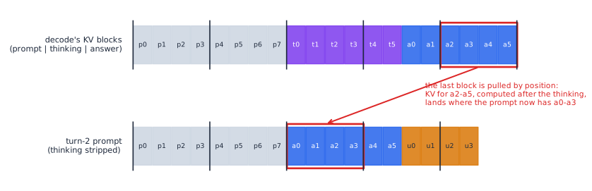
This is the difference between slow and wrong. A single server’s prefix cache identifies blocks by a hash chained over all the tokens before them. Change the history, and every later hash changes, so nothing incorrect can ever match; the cost is a cache miss and a recompute. Positional selection skips that check, so a changed history silently produces the wrong keys and values.
The issue’s suggested fix lives in the router: keep each conversation’s previous token IDs, compare them against the new prompt, and if they don’t line up, drop the cached transfer parameters and let prefill recompute. vLLM’s reference multi-turn proxy doesn’t do this yet: it keys turns only by a client-supplied conversation_id and reuses the previous turn’s transfer parameters on any hit, without comparing tokens. A commenter asks the natural follow-up: why throw everything away rather than reuse the longest matching prefix? The toy above answers it. The blocks before the first difference (the original prompt) are safe to reuse; everything after needs recomputing.
A maintainer adds the detail that widens the warning: many coding harnesses rewrite tool calls between turns, so this isn’t only about thinking traces. Any history that gets edited between turns triggers it.
That should sound familiar from my CLM review. Context Language Models edit their own context mid-conversation by design. Ordinary prefix caching survives that as a performance cost; positional KV reuse would turn it into wrong answers. And the review’s analysis of Suffix Cache Reuse found that most of its savings came from exactly this kind of reasoning-token stripping. It’s the same structural fact everywhere: reuse is only safe when what you reuse is checked against what the model will actually see.
What to do before turning bidirectional transfer on:
- Check your chat template. Does it drop past reasoning? Does your client or agent harness rewrite history (tool-call formats, compaction, summaries)?
- If either is true, verify in the router. Compare the new prompt’s token IDs with the previous turn’s, and reuse only up to the first difference.
- Or keep history stable. Use a template or mode that preserves reasoning across turns, where your model supports it.
- Or leave bidirectional transfer off for those workloads, and accept one-way recomputation as the price of correctness.
Running the GPU-less frontend
What “GPU-less” means, and why move the work at all
A serving system’s frontend is everything between an HTTP request and the token IDs a model consumes, and everything on the way back. We met its pieces earlier: chat templating, tokenization, detokenization, reasoning parsing, tool-call parsing. A GPU-less frontend simply runs those pieces on machines that have no GPU at all.
Think of a restaurant. The chefs are the GPUs: expensive, specialized, and the reason the place exists. The front of house takes orders in the customer’s language, writes them up as kitchen tickets, and later turns each plate into a description at the table. Nobody pays chefs to take orders. And once the front of house is a separate team, the kitchen only ever sees tickets.
In vLLM’s split, the ticket is a list of token IDs. The render tier writes it, the engine cooks from it, and the derender tier describes the result.
The guide’s point is that moving the work is “only part of it.” The bigger change is to the engine’s interface. Once the engine takes token IDs in and gives token IDs out, it no longer needs the chat template or the parsers. And the caller, whether a router, a trainer, or an evaluation harness, gets to see and use the exact token IDs. We walked through the three hops in miniature back in Claim 3; this section is about who benefits from seeing the tokens.
Who gains from seeing the real tokens
1. Routers that know where the cache is. With several replicas behind a load balancer, the best replica for a request is the one already holding the longest prefix of its KV cache, since that’s prefill work saved. But a prefix cache is keyed by token blocks, hashed in order from the very first token (the KV-caching refresher explains why). Text alone is a poor guide to that.
Here’s a router choosing between two replicas, first by comparing the user’s text, then by rendering the request and comparing token-block hashes:
# "A router can render a request, then pick a replica on prefix cache hits for the real prompt tokens
# rather than guessing from text." Two replicas, one new request: which replica already holds its KV?
import hashlib
from jinja2 import Template
from render_derender_toy import tokenize

BLOCK = 16
TEMPLATE = Template("{% for m in messages %}<|start|>{{ m.role }}\n{{ m.content }}<|end|>\n{% endfor %}<|start|>assistant\n")
DOC = "CONTRACT: The supplier shall deliver 400 units per month for 36 months at a fixed price. " * 4

def render(system, user):
    return tokenize(TEMPLATE.render(messages=[{"role": "system", "content": system},
                                              {"role": "user", "content": user}]))

def block_hashes(ids):
    h, out = "", []
    for i in range(0, len(ids) - len(ids) % BLOCK, BLOCK):
        h = hashlib.sha256((h + ",".join(map(str, ids[i:i + BLOCK]))).encode()).hexdigest()[:10]
        out.append(h)
    return out

# What each replica served last (and therefore holds in its prefix cache)
replicas = {
    "replica A": ("Be concise.",   DOC + "Q: what is the termination clause?"),
    "replica B": ("Be thorough.",  DOC + "Q: who pays for shipping?"),
}
new_system, new_user = "Be thorough.", DOC + "Q: what is the termination fee?"

# Router 1: guess from text -- compare the user's message with each replica's last message
def common_chars(a, b):
    n = 0
    while n < min(len(a), len(b)) and a[n] == b[n]: n += 1
    return n
text_pick = max(replicas, key=lambda r: common_chars(new_user, replicas[r][1]))

# Router 2: render to real token IDs, hash the blocks, count leading blocks each replica already holds
new_hashes = block_hashes(render(new_system, new_user))
def cached_prefix_blocks(r):
    held = set(block_hashes(render(*replicas[r])))
    n = 0
    while n < len(new_hashes) and new_hashes[n] in held: n += 1
    return n
token_pick = max(replicas, key=cached_prefix_blocks)

print(f"new request renders to {len(new_hashes)} full blocks of {BLOCK} tokens\n")
for r in replicas:
    print(f"{r}: same user text for {common_chars(new_user, replicas[r][1])} characters, "
          f"cached prefix = {cached_prefix_blocks(r)} blocks ({cached_prefix_blocks(r) * BLOCK} tokens)")
print(f"\ntext-guessing router picks : {text_pick}  -> reuses {cached_prefix_blocks(text_pick) * BLOCK} tokens")
print(f"token-hashing router picks : {token_pick}  -> reuses {cached_prefix_blocks(token_pick) * BLOCK} tokens")
print("The system prompt is rendered FIRST, so a different system prompt changes every block after it,"
      "\nhowever similar the user's text looks.")
new request renders to 25 full blocks of 16 tokens
replica A: same user text for 383 characters, cached prefix = 0 blocks (0 tokens)
replica B: same user text for 361 characters, cached prefix = 24 blocks (384 tokens)
text-guessing router picks : replica A -> reuses 0 tokens
token-hashing router picks : replica B -> reuses 384 tokens
The system prompt is rendered FIRST, so a different system prompt changes every block after it,
however similar the user's text looks.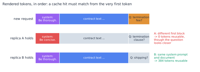
The text router picks replica A, because its last question looks closer, and reuses nothing. The chat template renders the system prompt first, and A’s is different, so every block after it differs too. The token router sees that and picks B, reusing 384 tokens of prefill.
Real routers face the same trap in subtler forms: template versions, tool definitions, a date stamped into the system prompt. A render tier that hands the router real token IDs removes the guessing.
2. Training and evaluation pipelines that need the exact tokens. Decoded text doesn’t always re-tokenize to the same IDs. Claim 3’s toy showed a model that sampled He + llo and got back a single different token on re-tokenizing Hello. For reinforcement learning, that’s not cosmetic. GRPO’s importance ratios (see the policy-gradients refresher) compare the probability of each token the model actually produced, so re-tokenized text computes ratios for tokens that were never sampled. The same holds for any evaluation that scores log-probabilities. Getting the IDs straight from the engine makes the training data exactly what happened.
3. Debugging and reproducibility. When a response looks wrong, the most useful artifact is the exact token sequence the model saw. My post on why temperature 0 isn’t deterministic is a reminder of how many things can differ between two “identical” runs; having the token IDs removes one whole category of them.
Multimodal preprocessing moves too
(The vision-encoder refresher appears earlier, before the encoder-disaggregation section: jump to it.)
From a JPEG to something a GPU can eat
The guide’s last point about the render tier is the one I find most interesting: multimodal preprocessing moves too.
A model never sees a JPEG. Before an image reaches the vision encoder (see the vision-encoder refresher), a model-specific processor prepares it:
- Decode the compressed file into raw pixels.
- Resize it to the grid the model expects; Qwen2-VL-style models round each side to a multiple of 28 pixels.
- Normalize each color channel into the range the encoder was trained on, which turns 8-bit pixels into floating-point numbers.
- Patchify the result into the patches the encoder consumes, and record metadata: how many patches, in what grid, so the language model knows how many visual tokens to expect and where they go in the prompt.
All of that is CPU work, the same kind as tokenization, so it belongs on the render tier.
The split pipeline
With encoder disaggregation from earlier in this post, the render tier now feeds two different destinations:
- To the encoder pool: the processed tensors, the full prepared pixels.
- To prefill: just the metadata, meaning the image’s hash and where its visual tokens go. Prefill doesn’t need pixels; it needs to know how many placeholder positions to reserve, and which cached embeddings to load from the encoder through the encoder-cache connector.
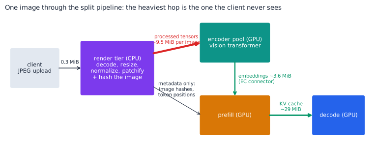
Why the payload balloons
The guide’s closing warning is that the processed payload can be much bigger than the source image, so request limits need sizing for it. Here’s how much bigger, following one photo hop by hop:
# "The processed payload can be much bigger than the source image." Follow one photo through the
# pipeline and weigh what travels at each hop.
import io
import numpy as np
from PIL import Image

MiB = 2 ** 20
# A photo-like test image: smooth gradients, shapes and a little noise compress like a real photo.
h, w = 1080, 1920
yy, xx = np.mgrid[0:h, 0:w]
img = np.stack([(xx / w * 200 + 30), (yy / h * 180 + 40), ((xx + yy) / (w + h) * 150 + 60)], axis=-1)
img[(xx - 1300) ** 2 + (yy - 500) ** 2 < 220 ** 2] = [220, 180, 60]
img[200:600, 300:700] = [70, 120, 200]
img = np.clip(img + np.random.default_rng(0).normal(0, 6, img.shape), 0, 255).astype(np.uint8)
buf = io.BytesIO(); Image.fromarray(img).save(buf, format="JPEG", quality=85)
jpeg = len(buf.getvalue())

# Hop 1 (render tier -> encoder): processed pixels.
plain = 640 * 640 * 3 * 4                                  # resize + normalize, float32
side = 644                                                 # Qwen2-VL-style: round to a multiple of 28 px
patches = (side // 14) ** 2                                # 14 x 14 pixel patches
qwen_style = patches * (3 * 2 * 14 * 14) * 4               # each patch duplicated along a time axis (x2), float32
# Hop 2 (encoder -> prefill): one embedding per merged visual token (2 x 2 patches -> 1 token)
tokens = patches // 4
embeddings = tokens * 3584 * 2                             # hidden size 3584, bf16
# For comparison: the KV cache those visual tokens become after prefill (Qwen2.5-7B-sized LM)
kv = tokens * 2 * 28 * 4 * 128 * 2

rows = [("source JPEG (what the client uploads)", jpeg),
        ("processed pixels, plain 640x640 float32", plain),
        ("processed pixels, Qwen2-VL-style patches", qwen_style),
        (f"embeddings for {tokens} visual tokens (bf16)", embeddings),
        ("KV cache for those tokens after prefill", kv)]
if __name__ == "__main__":
    print(f"{'stage':44s} {'size':>9s} {'x JPEG':>7s}")
    for name, size in rows:
        print(f"{name:44s} {size / MiB:7.2f} MiB {size / jpeg:6.0f}x")

    print("\nWire load between the render tier and the encoder pool:")
    for per_s in (10, 100):
        print(f"  {per_s:3d} images/s: JPEGs {per_s * jpeg * 8 / 1e9:6.2f} Gb/s  vs  processed tensors "
              f"{per_s * qwen_style * 8 / 1e9:5.1f} Gb/s")
    print("\nA request with 2 such images carries about "
          f"{2 * qwen_style / MiB:.0f} MiB of processed tensors -- past a 4 MiB default message limit many RPC stacks ship with.")
stage size x JPEG
source JPEG (what the client uploads) 0.27 MiB 1x
processed pixels, plain 640x640 float32 4.69 MiB 17x
processed pixels, Qwen2-VL-style patches 9.49 MiB 35x
embeddings for 529 visual tokens (bf16) 3.62 MiB 13x
KV cache for those tokens after prefill 28.93 MiB 106x
Wire load between the render tier and the encoder pool:
10 images/s: JPEGs 0.02 Gb/s vs processed tensors 0.8 Gb/s
100 images/s: JPEGs 0.23 Gb/s vs processed tensors 8.0 Gb/s
A request with 2 such images carries about 19 MiB of processed tensors -- past a 4 MiB default message limit many RPC stacks ship with.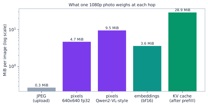
The JPEG is small because it’s compressed and stores 8-bit integers. Processing undoes both: it decompresses, and it converts every value to a 4-byte float. Some processors also duplicate each image along a time axis, so that images and video share one format. The result is a 35× jump: a 0.3 MiB upload becomes about 9.5 MiB on the hop between the render tier and the encoder. That hop is invisible to the client, which is exactly why the guide calls it out.
What to do about it:
- Size the internal hops, not just the public API. An upload limit of a few megabytes says nothing about the render-to-encoder message, which can be 30–40 times larger. Many RPC stacks ship with a 4 MiB default message limit, and a request with two such images already carries about 19 MiB of processed tensors.
- Budget the network. At 100 images per second, the processed tensors need about 8 Gb/s between the tiers, against 0.2 Gb/s for the original JPEGs.
- Consider the trade-offs. Sending pixels in 16-bit floats halves the payload. Sending the compressed image and preprocessing next to the encoder saves the network but puts CPU work back on the GPU box, the very thing this split tries to avoid.
- Let the hash do its job. The render tier hashes each image, so a repeated image (a logo, a product photo, a common diagram) can skip both the heavy hop and the encoder entirely through the encoder cache.
Text-only requests, meanwhile, never touch any of this. That is the quiet win of the whole design.
Putting it all together
The guide is practical, and it rewards being read with a calculator in hand. Here’s what I take from it, in order of how much it changes how I’d build a serving stack:
- Optimize goodput, and choose its targets carefully. Disaggregation doesn’t raise throughput. It keeps requests inside their latency targets as load climbs. Measured against an average per-token target it looks good; against a worst-gap target, the one users actually feel, it’s often the only design that works at all.
- One server does three jobs that interfere. Prefill is compute-bound, decode is memory-bound, and the frontend is CPU work. A prefill chunk riding in a decode step is the stutter users see, and the guide’s own p99 of 169 ms matches one 2,048-token chunk almost exactly.
- Every split is a cut through the model, priced by what crosses it. Embeddings cross once per image, the KV cache once per request, and attention-to-expert traffic on every step. The deeper the cut, the faster the interconnect has to be.
- The handoff decides whether P/D pays. The KV cache is big in bytes but small relative to the compute that produces it. Streamed layer by layer it costs almost nothing; sent late through a slow path, it costs seconds on every first token. Measure it before anything else.
- The frontend split changes the interface, not just the bill. An engine that speaks token IDs lets routers find real cache hits, lets trainers and evaluators use the exact tokens, and moves image preprocessing (and its 35× payload) onto cheap, separately scaled CPUs.
- Reuse is only safe when it’s checked. Multi-turn reuse is a big win for chat and agents. But whenever history changes between turns (stripped reasoning, rewritten tool calls, self-editing contexts like the CLM paper’s), positional reuse turns a performance shortcut into wrong answers. Verify tokens before you reuse KV.
The guide’s remaining sections cover deploying the render tier, putting both splits together, who runs this in production, and what’s still being built. The original is worth reading for the commands and configuration details I’ve deliberately left out here.
References
The sources reviewed
- Hickey, M. (2026). Taking vLLM Apart: A Practical Guide to Disaggregated Serving. vLLM Blog. https://vllm.ai/blog/2026-09-29-disaggregated-serving-guide
- Benveniste, D. (2026). LinkedIn post on vLLM’s disaggregated-serving guide, whose one-scenario framing inspired this post. https://www.linkedin.com/posts/damienbenveniste_vllms-new-disaggregated-serving-guide-makes-share-7511816453915074561-DA0x/
- Gordić, A. (2025). Inside vLLM: Anatomy of a High-Throughput LLM Inference System. vLLM Blog. https://vllm.ai/blog/2025-09-05-anatomy-of-vllm
Related vLLM posts
- vLLM Multimodality Workstream (2025). Encoder Disaggregation for Scalable Multimodal Model Serving. https://vllm.ai/blog/2025-12-15-vllm-epd
- AFD Plugin Contributors (2026). Announcing vLLM AFD Plugin: Disaggregating Attention and FFN for Flexible MoE Serving. https://vllm.ai/blog/2026-07-23-vllm-afd-plugin
- Lucchesi, N., Hu, Z., and the vLLM team (2026). Disaggregated Serving for Hybrid SSM Models in vLLM. https://vllm.ai/blog/2026-04-21-hybrid-ssm-disagg
- vLLM Blog (2026). vLLM x AgentX: Optimizing for Real-World Agentic Serving. https://vllm.ai/blog/2026-09-08-vllm-agentx
vLLM documentation and code (Apache-2.0)
- Disaggregated Prefilling (experimental). https://docs.vllm.ai/en/latest/features/disagg_prefill/
- NixlConnector Usage Guide, including “Bidirectional KV Transfer (Multi-turn)“. https://docs.vllm.ai/en/stable/features/nixl_connector_usage/
- vLLM issue #43094. [Bug][PD] Bidirectional KV transfer produces incorrect results when reasoning traces are stripped between turns. https://github.com/vllm-project/vllm/issues/43094
- vLLM source code. https://github.com/vllm-project/vllm
Papers
- Licker, N., Hu, K., Zaytsev, V., and Chen, L. (2026). fabric-lib: RDMA Point-to-Point Communication for LLM Systems. MLSys 2026. https://arxiv.org/abs/2510.27656. A portable RDMA library from Perplexity, used in production for KV-cache transfer, RL weight updates, and MoE dispatch/combine. RDMA in two lines: remote direct memory access lets a network card read or write another machine’s memory, GPU memory included, without involving either machine’s CPU or operating system on the data path. That’s what makes 400 Gb/s, microsecond-latency transfers of KV caches and expert activations possible.
Related posts on this blog
- Context Language Models, Dissected: prefix caching, Suffix Cache Reuse, and why edited histories break reuse.
- Tiny CLM: GRPO on a small model, and why exact token IDs matter in training.
- Inside SGLang: Anatomy of a High-Performance Structured LLM Inference System.
- SGLang Deep Dive: Inside SGLang.
- Why Temperature=0 Doesn’t Mean Deterministic LLM Inference.
- EAGLE-3: Soaring Beyond Speed, on speeding up decode.
- From Cloud to Couch: Supercharging SmolLM2 Inference with HeadInfer, Gemlite, and SGLang, on KV-cache memory on local hardware.
All figures are original. All numbers in this post come from the programs shown or from the cited sources.